ぐるぐる
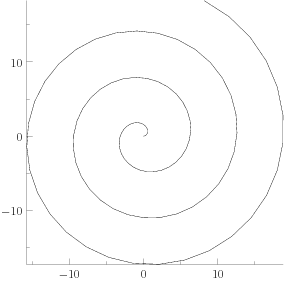
spiral.asy:
size(10cm);

import graph;

draw(polargraph(identity, 0, 20));

xaxis(Bottom(), LeftTicks());
yaxis(Left(), RightTicks());
ルーローの三角形を回したときの動作を図示するとき、どういう間隔で状態を描いたらいいか。
たとえば、接地している位置が一定間隔になるように描くのは望ましくない。角が地面に刺さっているときは接地している位置がしばらく変わらないので、その間の状態変化を図示できない。
ましな方法はいくつか考えられるが、重心の横方向の移動が一定間隔になるように描くことを考えた。
が、これをやるにはどうも x + r/sqrt(3) * sin(pi/6-x/r) = y を x について解く必要があって、解けなくて困った。(ちなみに Wolfram Alpha でも解けなかった)
結局、Asymptote には Newton 法の実装が入っているので、それを使ってなんとか描けた。
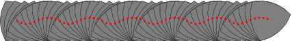
reuleaux-center-movement.asy:
size(15cm);

pair a = (0,1);
pair b = rotate(120)*a;
pair c = rotate(-120)*a;
real r = length(a-b);

path tri = arc(c,r,120,180)--arc(a,r,240,300)--arc(b,r,0,60)--cycle;

real outlinelen = arclength(tri);
real edgelen = outlinelen/3;

real cyclelen = pi*r/3;

typedef real realfunc(real);
realfunc move1(real y) {
  return new real(real x) {
    return x + r/sqrt(3) * sin(pi/6-x/r) - y;
  };
}

real move1prime(real y) {
  return 1 + r/sqrt(3) * cos(pi/6-pi/r);
}

transform ms[];
for (real x = 0.001; x < cyclelen*6; x += cyclelen/10) {
  int n = floor(x/cyclelen);
  real x2 = fmod(x, cyclelen);
  if (x2 < (pi/3-1/sqrt(3))*r) {
    real x3 = newton(move1(x2+r/(2*sqrt(3))), move1prime, x2);
    real t = arctime(tri, x3);
    pair p = point(tri, t);
    pair d = dir(tri, t);
    transform mat = shift(n*edgelen+x3,0)*rotate(-degrees(atan2(d.y,d.x)))*shift(-p);
    ms.push(mat);
  }
  else {
    real x3 = x2 - (pi/3-1/(2*sqrt(3)))*r;
    real deg = degrees(asin(sqrt(3)*x3/r));
    transform mat = shift((n+1)*edgelen)*rotate(-60-deg)*shift(-c);
    ms.push(mat);
  }
}

for (int i = 0; i < ms.length; ++i)
  filldraw(ms[i]*tri, gray);
for (int i = 0; i < ms.length; ++i)
  dot(ms[i]*(0,0), red);
buildcycle というのを見つけて、使ってみると輪郭線をつけてもこれで描けた。
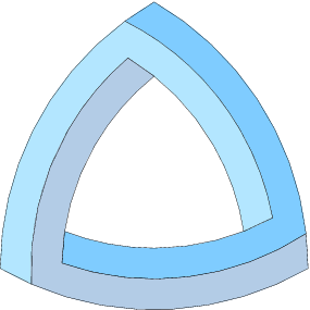
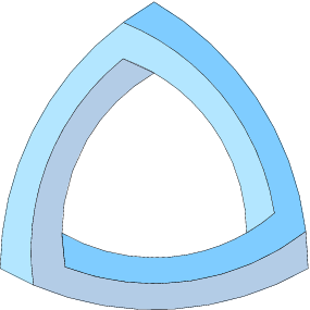
reuleaux-penrose-triangle-buildcycle.asy:
size(10cm,10cm);

pair a = (0,1);
pair b = rotate(120)*a;
pair c = rotate(-120)*a;

real len3 = length(a-b);
real len2 = len3 * 0.9;
real len1 = len3 * 0.8;

path p = buildcycle(
  arc(b, len3, 0, 80),
  arc(c, len3, 90, 150),
  arc(b, len2, 80, 0),
  arc(a, len1, -60, -120),
  arc(c, len1, 150, 240),
  arc(a, len2, -120, -30));

filldraw(p, rgb(0.5,0.8,1));
filldraw(rotate(120)*p, rgb(0.7,0.9,1));
filldraw(rotate(240)*p, rgb(0.7,0.8,0.9));
buildcycle の説明はマニュアルには
path buildcycle(... path[] p);
  This returns the path surrounding a region bounded by
  a list of two or more consecutively intersecting paths,
  following the behaviour of the MetaPost buildcycle command.
と、1文しか書いてなくてしかも MetaPost を参照していてよくわからないのだが、複数の曲線を与えると、その交点でそれらの部分曲線をつないで閉曲線を作る、というもののようだ。
図で説明すると以下のようなかんじ。p1, p2, p3, p4, p5, p6 という円弧 (のそれぞれ一部分) をつないで、青く塗られた部分の領域を囲う閉曲線を構成する。
ユーザの立場からは、交点を自分で計算する必要がないのが良い。
しかし、複数の曲線から取り出せる閉曲線が複数あったらどうなるのか。仕様がいまひとつ曖昧な気はする。
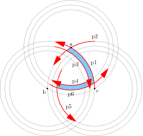
reuleaux-penrose-triangle-structure.asy:
size(10cm);

pair a = (0,1);
pair b = rotate(120)*a;
pair c = rotate(-120)*a;

real len3 = length(a-b);
real len2 = len3 * 0.9;
real len1 = len3 * 0.8;

path p1 = arc(b, len3, 0, 80);
path p2 = arc(c, len3, 90, 150);
path p3 = arc(b, len2, 80, 0);
path p4 = arc(a, len1, -60, -120);
path p5 = arc(c, len1, 150, 240);
path p6 = arc(a, len2, -120, -30);

path p = buildcycle(p1, p2, p3, p4, p5, p6);

fill(p, rgb(0.5,0.8,1));

draw(shift(a)*scale(len1)*unitcircle, gray);
draw(shift(a)*scale(len2)*unitcircle, gray);
draw(shift(a)*scale(len3)*unitcircle, gray);
draw(shift(b)*scale(len1)*unitcircle, gray);
draw(shift(b)*scale(len2)*unitcircle, gray);
draw(shift(b)*scale(len3)*unitcircle, gray);
draw(shift(c)*scale(len1)*unitcircle, gray);
draw(shift(c)*scale(len2)*unitcircle, gray);
draw(shift(c)*scale(len3)*unitcircle, gray);

pen pen = red+1.2;
draw(p1, pen, EndArrow); label("p1", point(p1, length(p1)/3), NE);
draw(p2, pen, EndArrow); label("p2", point(p2, length(p2)/2), N);
draw(p3, pen, EndArrow); label("p3", point(p3, length(p3)/2), SW);
draw(p4, pen, EndArrow); label("p4", point(p4, length(p4)/2), NE);
draw(p5, pen, EndArrow); label("p5", point(p5, length(p5)/5*4), NE);
draw(p6, pen, EndArrow); label("p6", point(p6, length(p6)/2), S);

dot(a); label("a", a, N);
dot(b); label("b", b, SW);
dot(c); label("c", c, SE);
Asymptote をいくらか使ってみた感想:
- まともな関数型言語とも見える
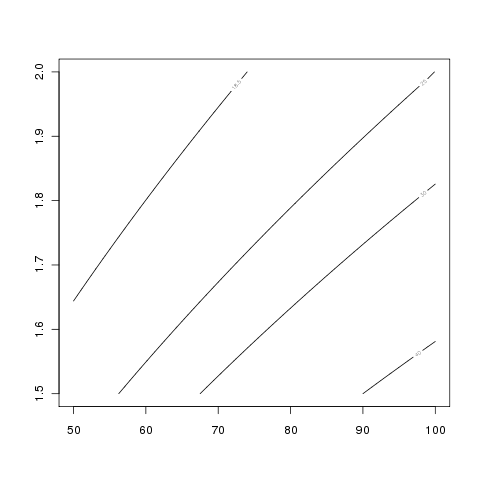
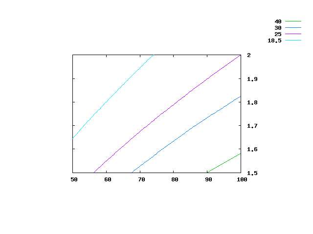
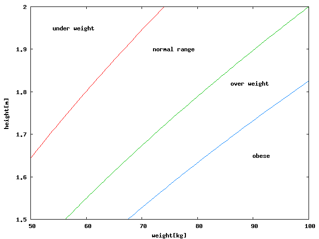
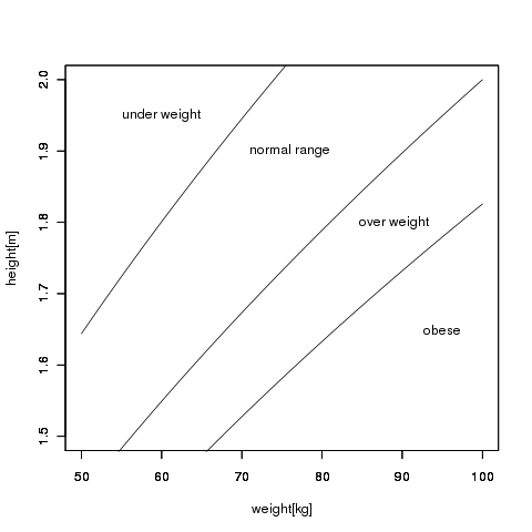
- gnuplot ほど簡単にグラフを描けるわけではない
- 厄介な作図をするのに向いている
あと、マニュアル に
Asymptote is the only language we know of that treats functions as variables,
but allows overloading by distinguishing variables based on their signatures.

Asymptote は関数を変数として扱う言語の中で、我々が知る限り唯一、
変数をそのシグネチャによって区別してオーバーロードできる言語である。
と書いてある。
% asy
Welcome to Asymptote version 1.43 (to view the manual, type help)
> int x, x()
> x = new int() { return 2; }
> x = 3
> x()
2
> x+0
3
> x()
2
> x+0
3
> x
-: 1.1: warning: writing overloaded variable 'x'
3
>
x という名前の、int な変数と、引数なしで int を返す関数が両方同時に存在し、使い方によって選ばれる。選べないときもあるが。
後から、int 引数をとって int を返す関数 x を加えても、いままであった x は残る。
> int x(int)
> x = new int(int v) { return v; }
> x()
2
> x(10)
10
> x()
2
> x+0
3
こだわりが感じられる。


