天泣記

2016-10-13 (Thu)

#1 Hash は O(1) か

hash table の lookup の実行時間は O(1) である。が、本当にそうなのか測ってみよう。

% ./miniruby -v
ruby 2.4.0dev (2016-10-12 trunk 56401) [x86_64-linux]
% ./miniruby -e '
def fmt(n) "%10d" % n end
puts "n,t[s]"
n = 1
h = {}
while n < 1e8
  h[fmt(h.size)] = true while h.size < n
  k = fmt(rand(n))
  GC.start
  GC.disable
  h[k]
  t1 = Process.clock_gettime(Process::CLOCK_THREAD_CPUTIME_ID)
  h[k]
  t2 = Process.clock_gettime(Process::CLOCK_THREAD_CPUTIME_ID)
  GC.enable
  t = t2-t1
  puts "#{n},#{t}"
  STDOUT.flush
  n = (n*1.1).to_i+1
end' > hash-lookup-time.csv
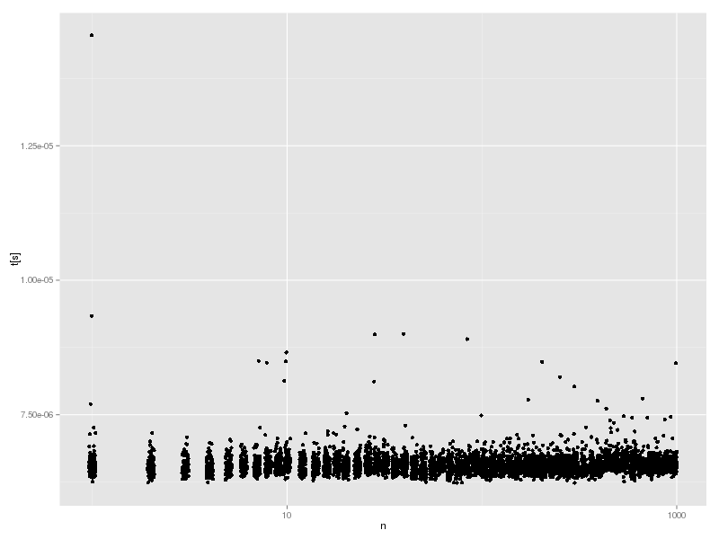
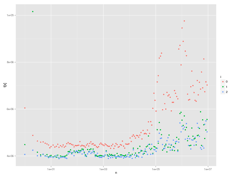
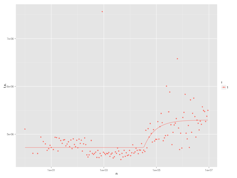
グラフにしてみる。

hash-lookup-time.R:

library(ggplot2)
d <- read.csv("2016-10/hash-lookup-time.csv")
p <- ggplot(d, aes(n, t.s.)) +
  geom_point() +
  scale_x_log10() +
  scale_y_continuous("t[s]", limits=c(0,2e-6))
print(p)

hash-lookup-time.png

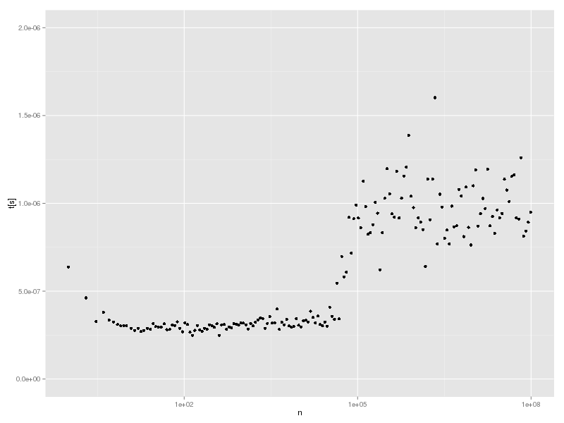
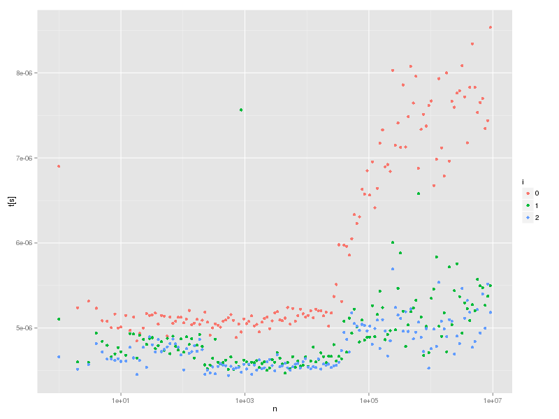
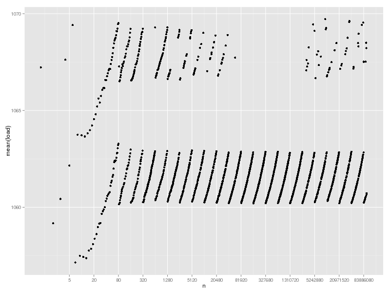
まぁ定数時間には見えない。n (Hash の要素数) が小さいと遅いし、n が大きくてもあるところから遅くなる。

なにが起きているのかな。

大きい方については、キャッシュに入らないからじゃないかな、と感じるのだが、確認したわけではない。

#2 PAPI

キャッシュに入らないから、というのを確認するにはどうしたらいいかといえば、キャッシュミスを数えればいいわけである。

しかし、どうしたら数えられるか知らなかったので、調べて見たところ、 PAPI というライブラリが使えそうである。Debian package にもなっている。

Ruby binding を作った人もいるようだ: PAPI gem

これらは以下のように install できる。

sudo aptitude install papi-tools
gem install PAPI

gem のドキュメントはほとんどないが、適当に試したところ、以下のようにすれば動くようだ。

% ./ruby -rPAPI -e '
evset = PAPI::EventSet.new
evset.add_named(%w[PAPI_TOT_INS PAPI_L1_DCM])
evset.start
3 ** 100
p evset.stop
evset.start
3 ** 1000
p evset.stop
'
[8689, 370]
[29572, 676]

PAPI::EventSet オブジェクトを作って、add_named メソッドで数えたいイベントを指定して、start メソッドで数え始めて、stop メソッドで終了して結果を返す。

上の例だと、3 ** 100 を実行するのに、PAPI_TOT_INS が 8689回、PAPI_L1_DCM が 370回起きている。つまり、8689回インストラクションが実行され、L1 data cache の miss が 370回起きている。

3 ** 1000 を実行するのには、PAPI_TOT_INS が 29572回、PAPI_L1_DCM が 676回である。

数えられるイベントのリストは papi_avail コマンドや papi_native_avail コマンドで表示できる。(アーキテクチャによって異なる)

papi_avail では上記の PAPI_TOT_INS と PAPI_L1_DCM を含め PAPI が定義した(比較的)ポータブルなイベントが出てくる。

papi_native_avail はいろいろと生のイベントが出てくる。ix86arch::LLC_MISSES とか、perf::INSTRUCTIONS とか。perf:: というのは、名前からするともしかして perf のメカニズムを使っているのかもしれない。(PAPI はイベントを数えるいろいろなものを統一的に扱うフレームワークなので、perf を扱えてもおかしくない。)

#3 大きい Hash が遅くなる理由

大きい Hash のが遅くなるのを、PAPI を使っていろいろ試したところ、どうも、TLB miss が原因のように思われる。

% ./ruby -rPAPI -e '
events = %w[PAPI_TOT_INS PAPI_TOT_CYC PAPI_RES_STL PAPI_TLB_DM]
evset = PAPI::EventSet.new
evset.add_named(events)
def fmt(n) "%10d" % n end
puts "n,t[s],#{events.join(",")}"
n = 1
h = {}
while n < 1e7
  h[fmt(h.size)] = true while h.size < n
  k = fmt(rand(n))
  GC.start
  GC.disable
  h[k]
  t1 = Process.clock_gettime(Process::CLOCK_THREAD_CPUTIME_ID)
  evset.start
  h[k]
  evrec = evset.stop
  t2 = Process.clock_gettime(Process::CLOCK_THREAD_CPUTIME_ID)
  GC.enable
  t = t2-t1
  puts [n,t,*evrec].join(",")
  STDOUT.flush
  n = (n*1.1).to_i+1
end' > hash-lookup-tlb.csv

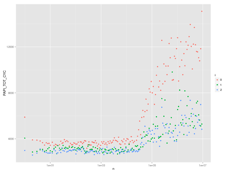
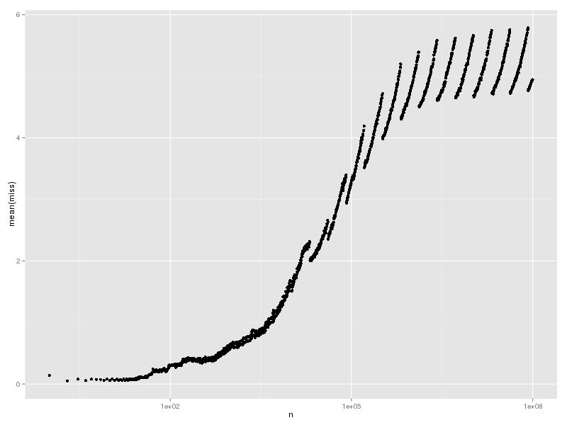
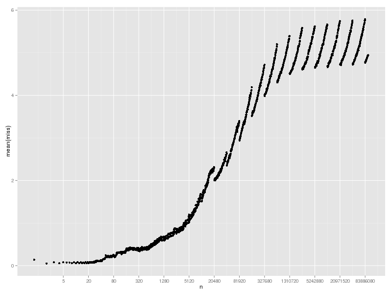
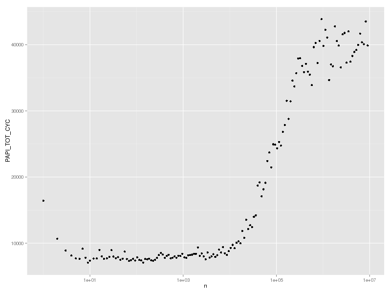
まず、PAPI_TOT_CYC (Total cycles) をグラフにすると、だいたい実行時間と似た形になることがわかる。(1e8 まで調べるのは時間がかかるので、1e7 までにした)

hash-lookup-totcyc.png

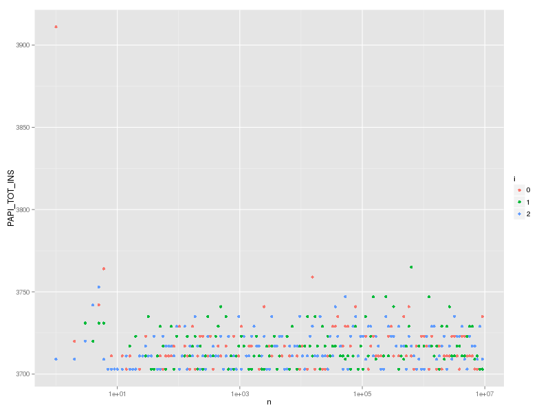
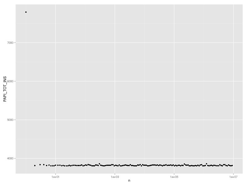
次に、PAPI_TOT_INS (Instructions completed) をグラフにすると、これは一定なことが確認できる。つまり、遅くなっていても、実行した命令の数は変わっていないのだ。

hash-lookup-totins.png

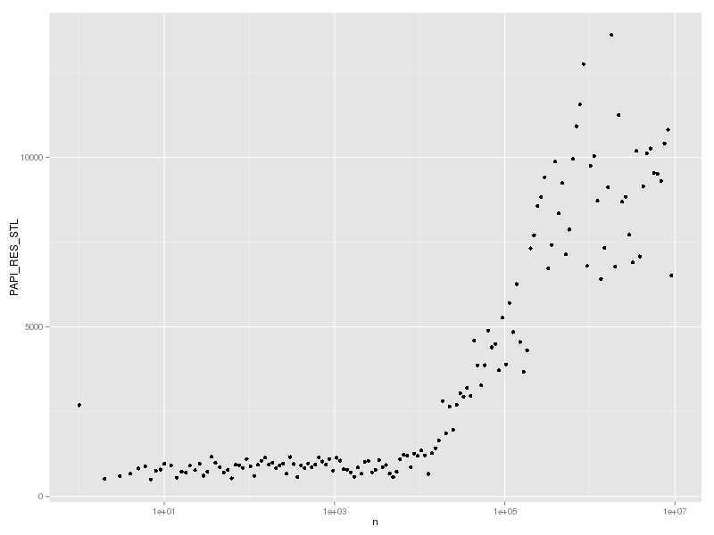
実行命令数が変わっていないのに実行時間が増えているということは、CPUが動いていない時間が増えているということである。そこで、PAPI_RES_STL (Cycles stalled on any resource) をグラフにすると、実際にストールしているサイクル数が増えていることがわかる。

hash-lookup-resstl.png

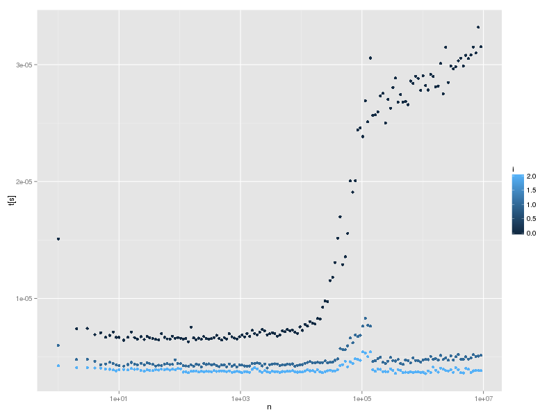
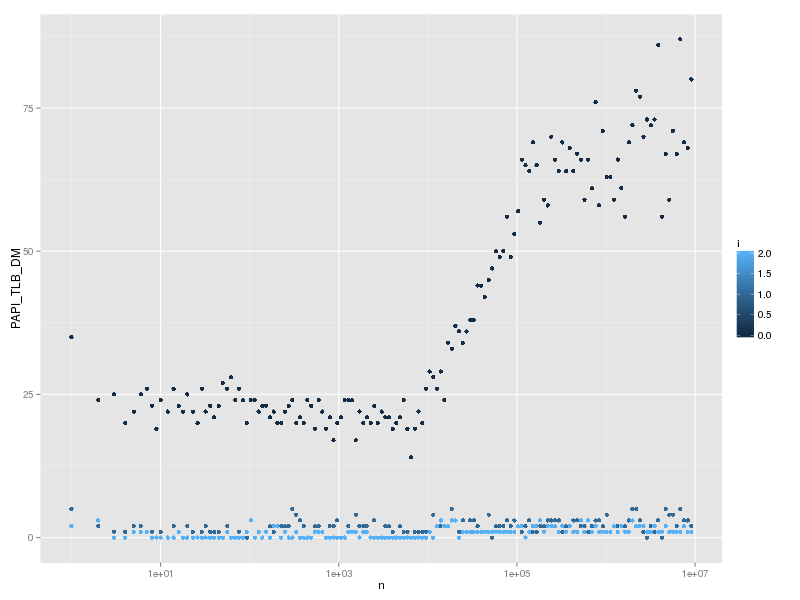
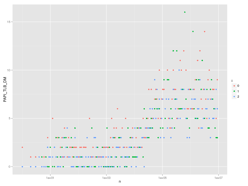
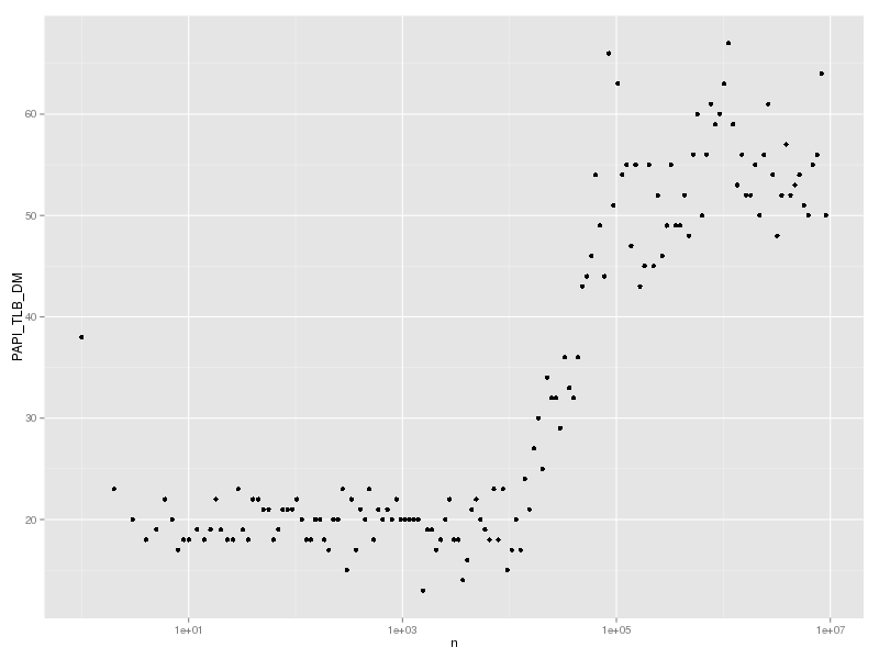
では stall が増える原因はなにかというと、おそらく TLB miss と思われる。これは PAPI_TLB_DM (Data translation lookaside buffer misses) で数えられる。これは実行時間や PAPI_TOT_CYC とよく似た形になっている。

hash-lookup-tlbdm.png

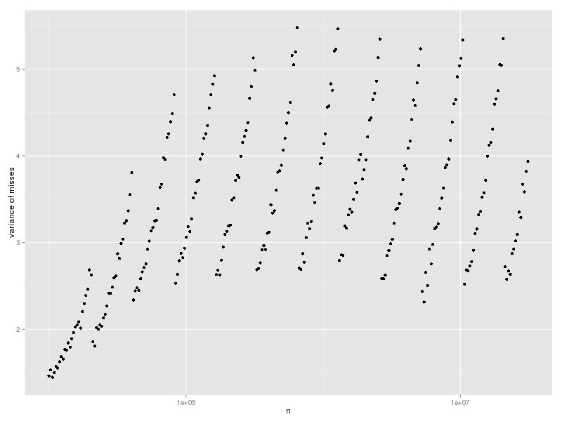
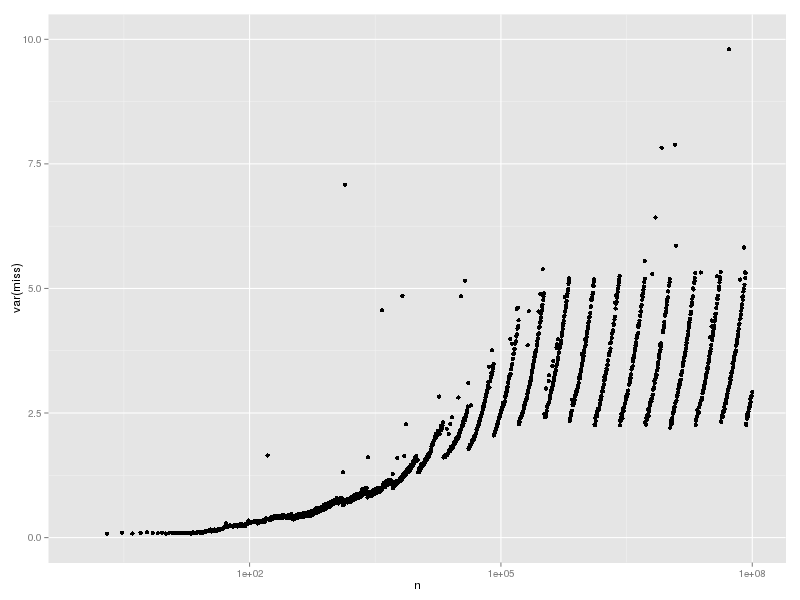
なお、cache miss も同じように測定できる。

% ./ruby -rPAPI -e '
events = %w[PAPI_L1_DCM PAPI_L2_DCM PAPI_L3_TCM]
evset = PAPI::EventSet.new
evset.add_named(events)
def fmt(n) "%10d" % n end
puts "n,t[s],#{events.join(",")}"
n = 1
h = {}
while n < 1e7
  h[fmt(h.size)] = true while h.size < n
  k = fmt(rand(n))
  GC.start
  GC.disable
  h[k]
  t1 = Process.clock_gettime(Process::CLOCK_THREAD_CPUTIME_ID)
  evset.start
  h[k]
  evrec = evset.stop
  t2 = Process.clock_gettime(Process::CLOCK_THREAD_CPUTIME_ID)
  GC.enable
  t = t2-t1
  puts [n,t,*evrec].join(",")
  STDOUT.flush
  n = (n*1.1).to_i+1
end' > hash-lookup-cache.csv

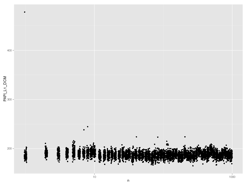
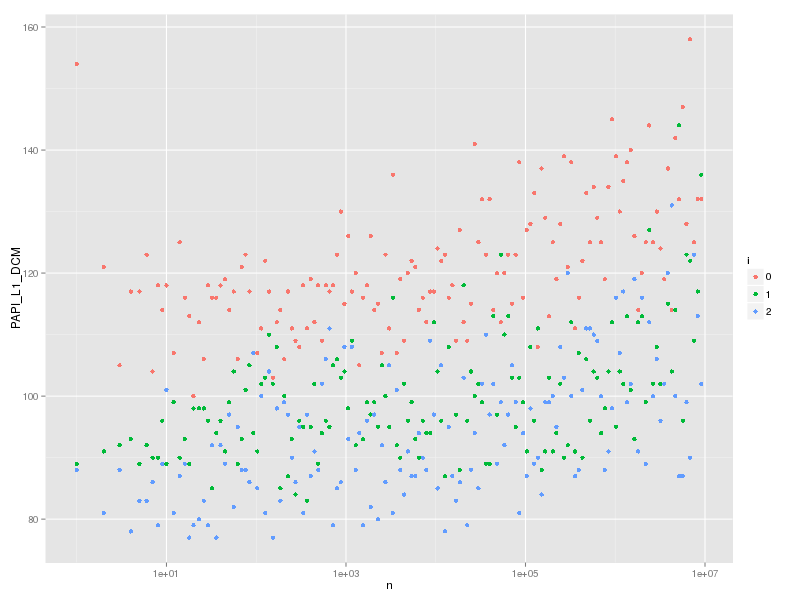
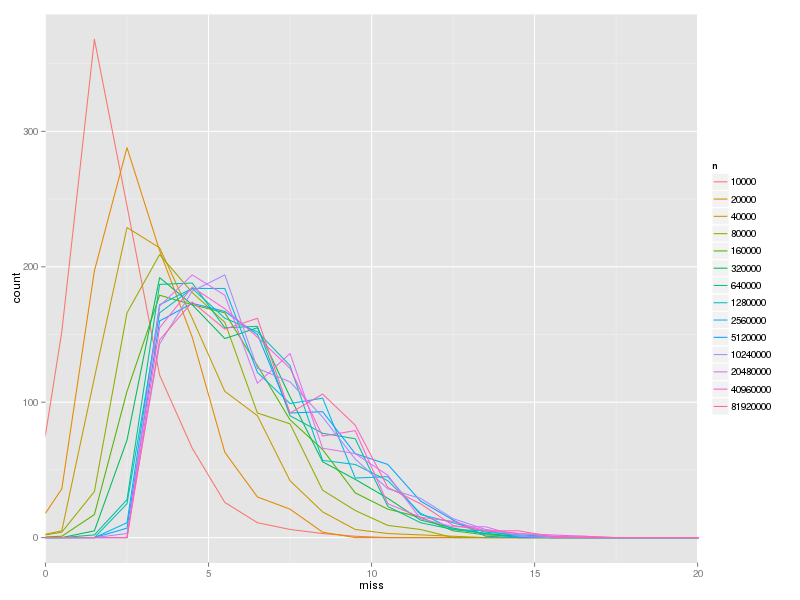
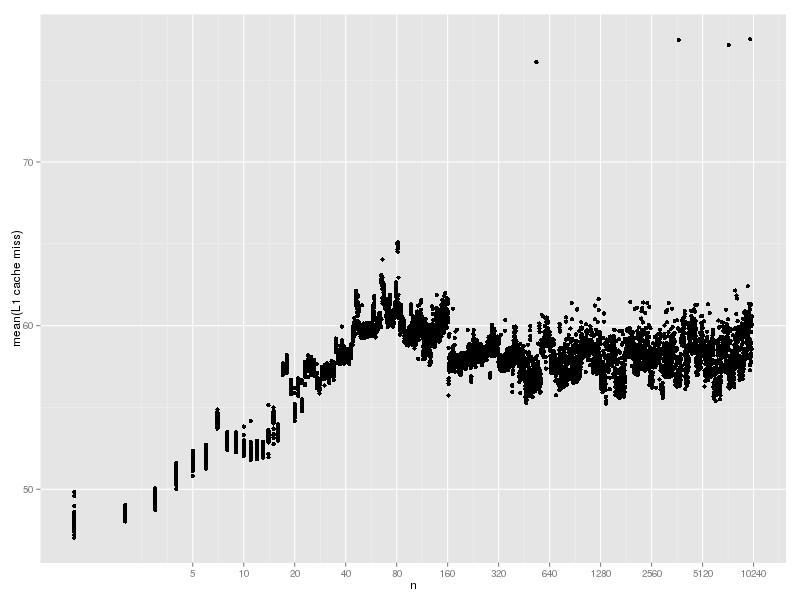
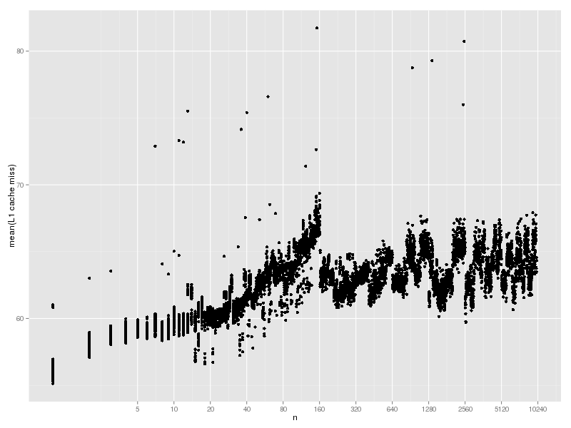
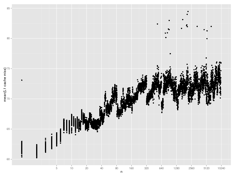
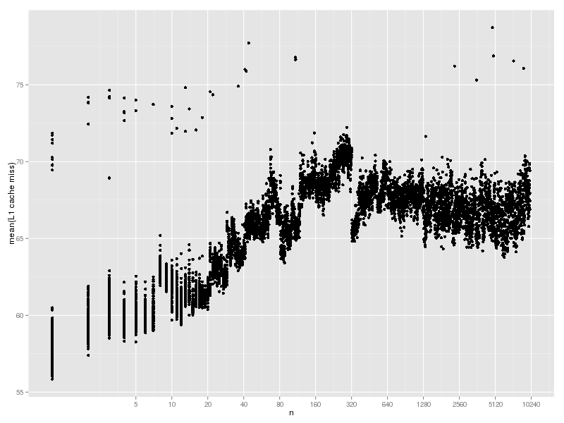
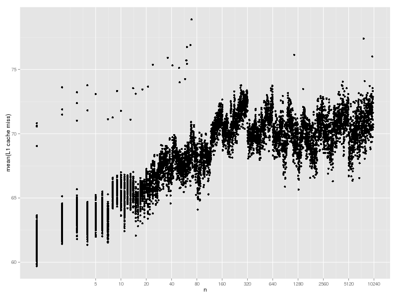
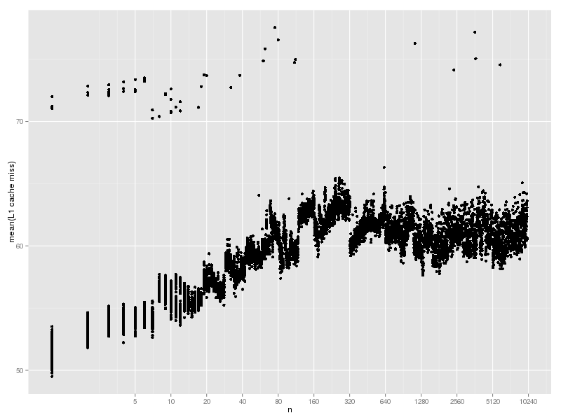
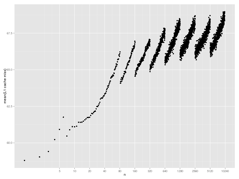
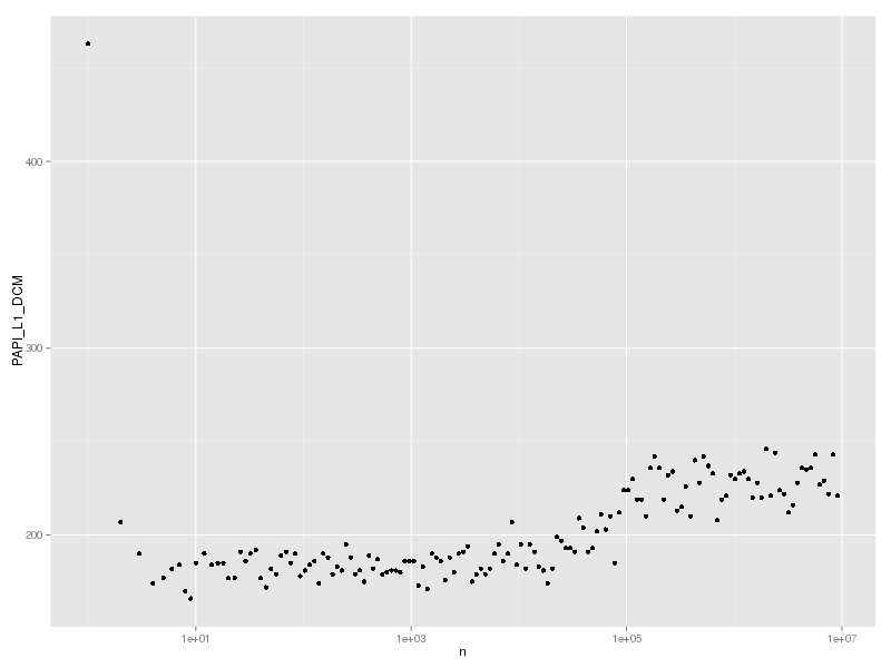
PAPI_L1_DCM (Level 1 data cache misses) は以下のようになる。

hash-lookup-l1dcm.png

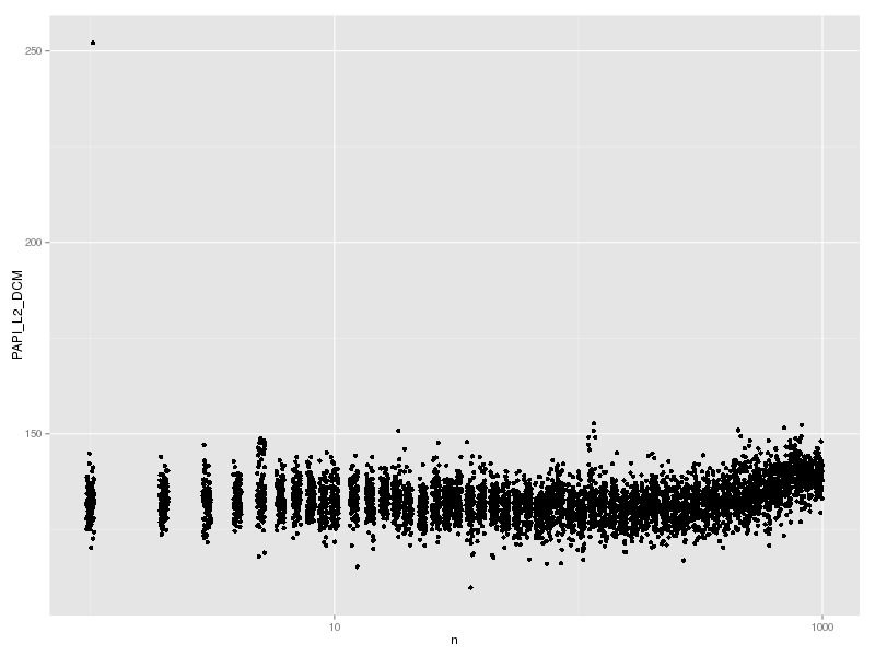
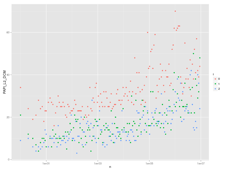
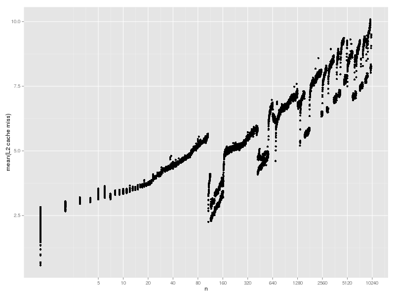
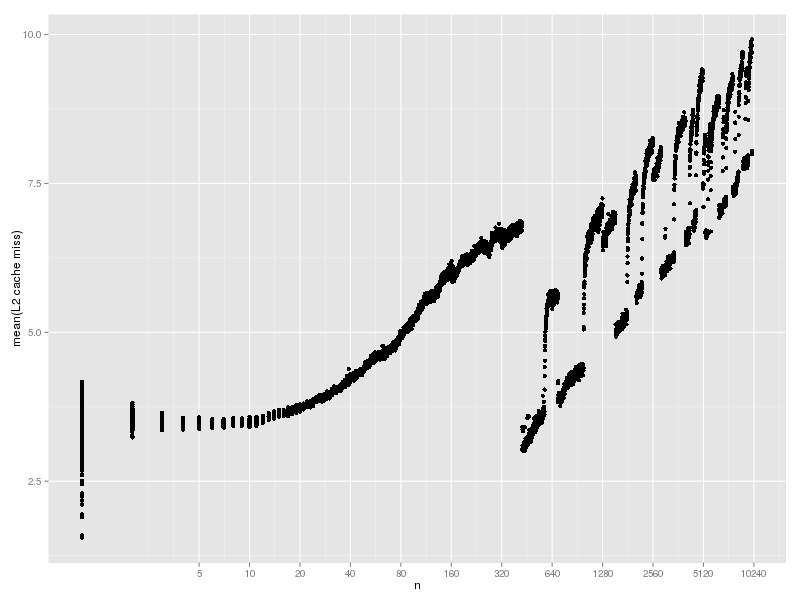
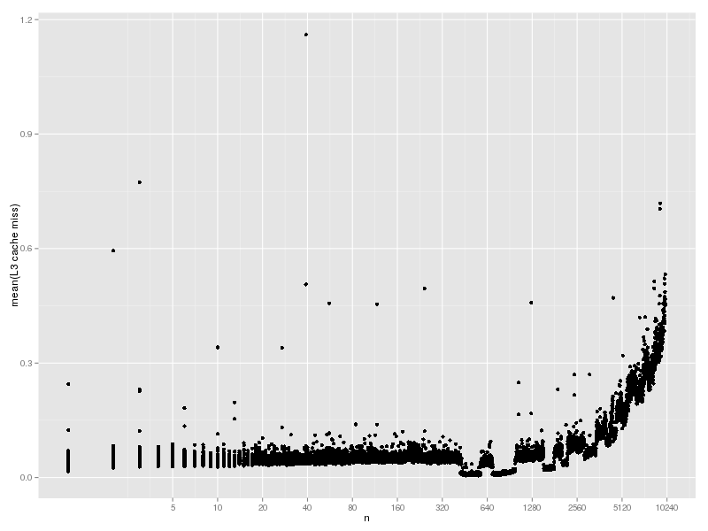
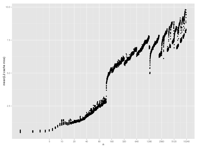
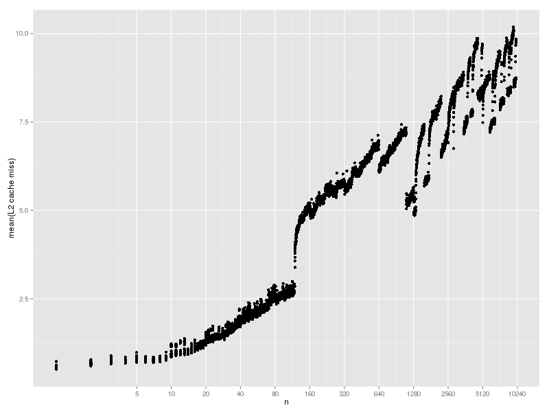
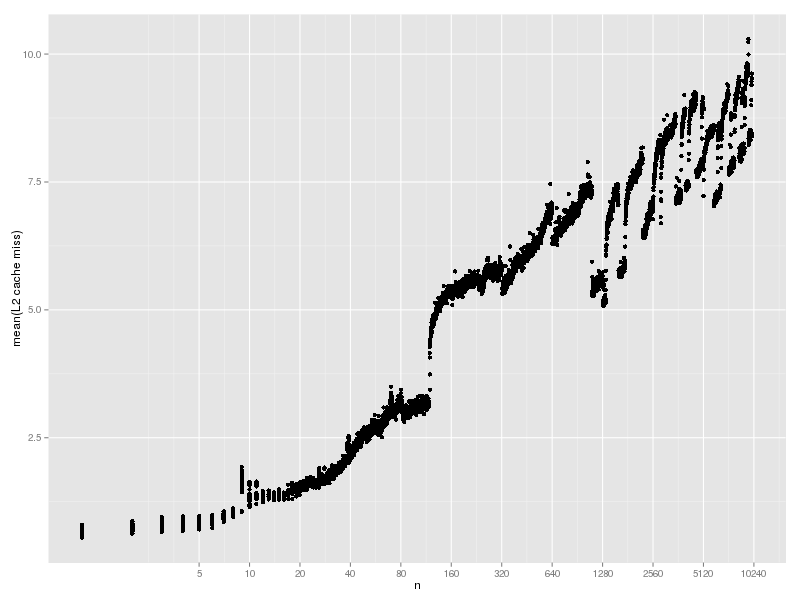
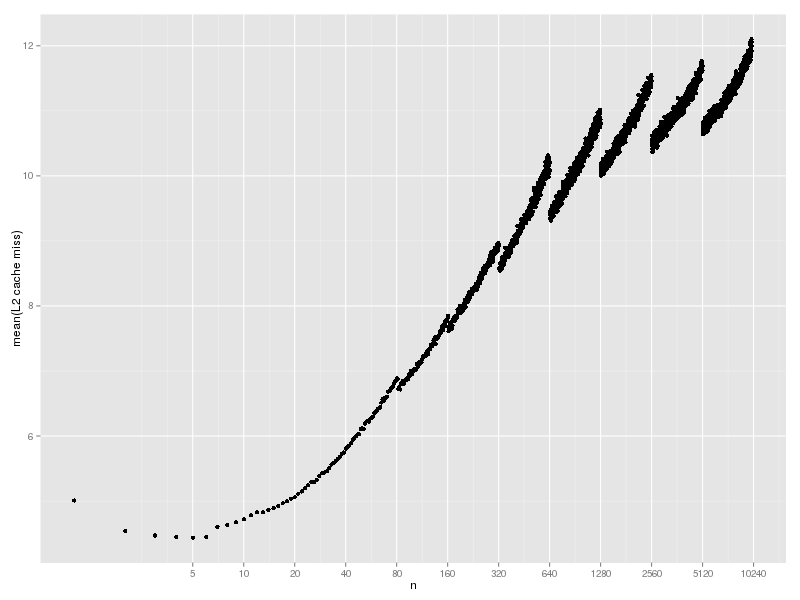
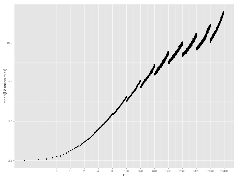
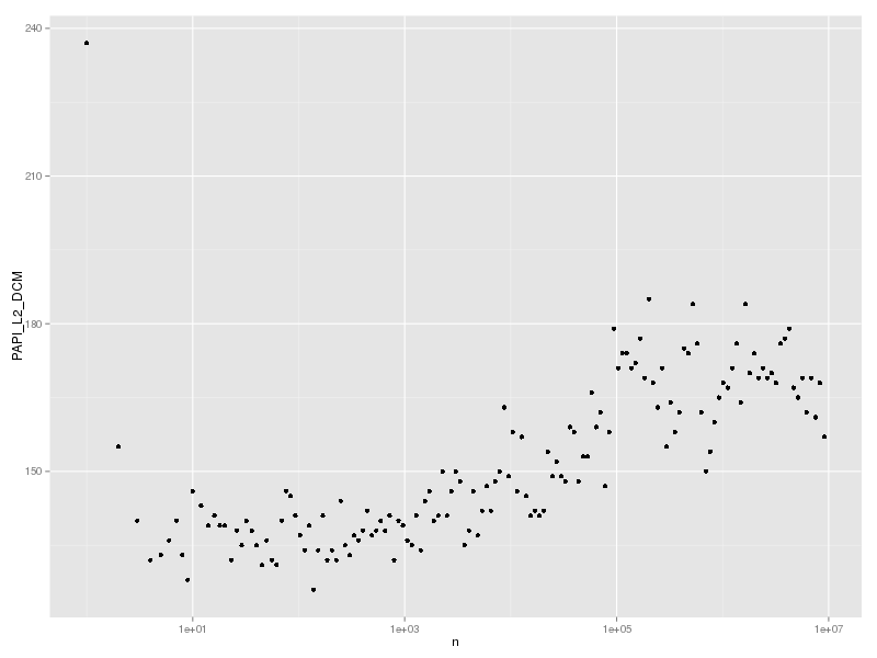
PAPI_L2_DCM (Level 2 data cache misses)

hash-lookup-l2dcm.png

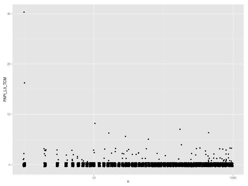
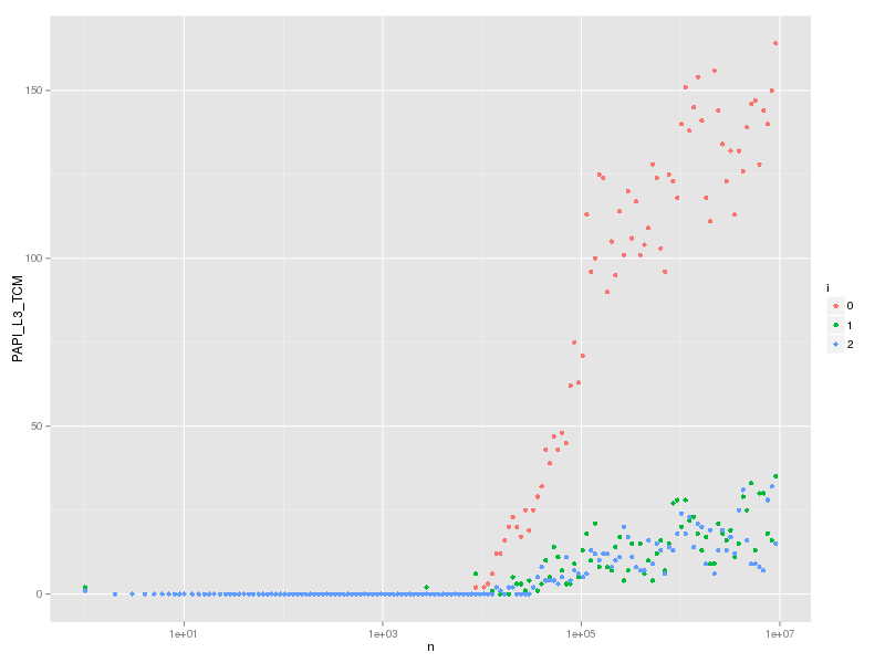
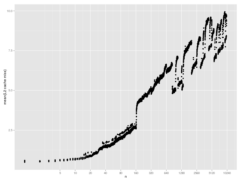
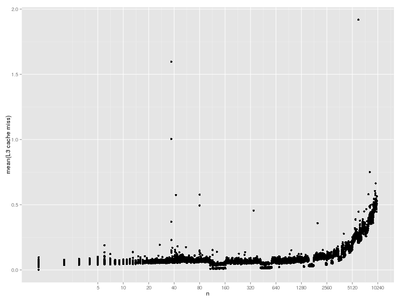
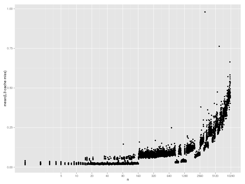
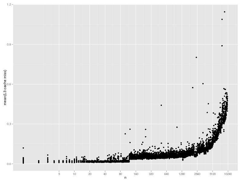
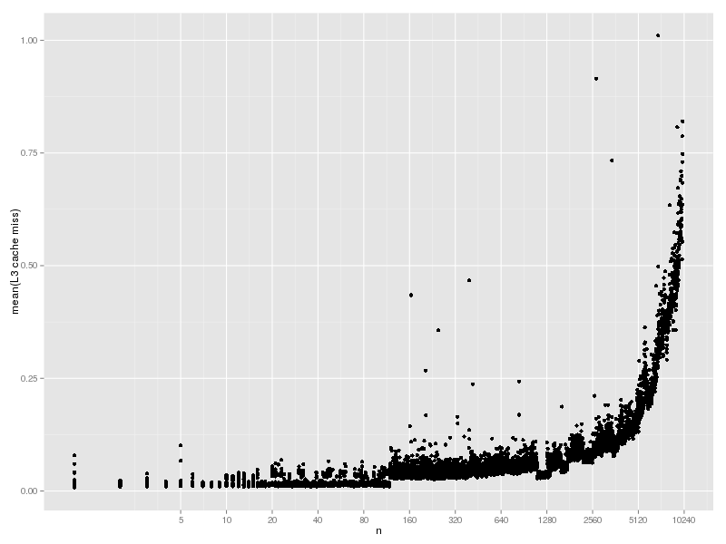
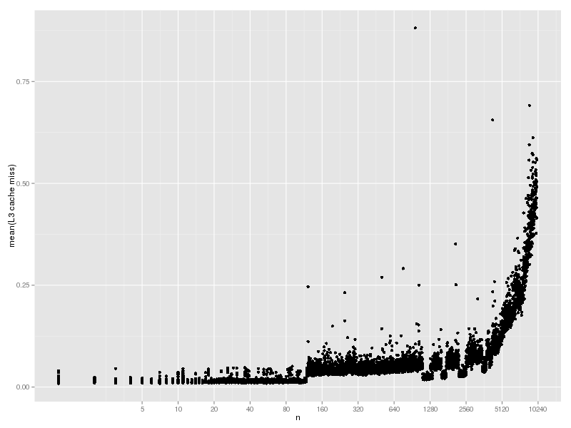
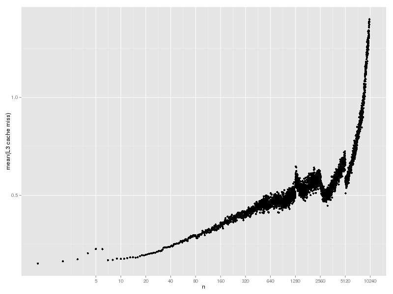
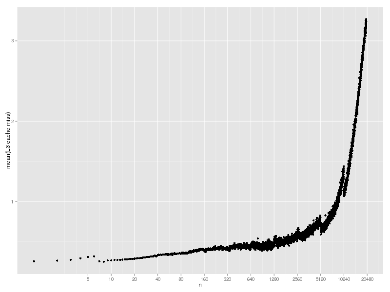
PAPI_L3_TCM (Level 3 cache misses)

hash-lookup-l3tcm.png

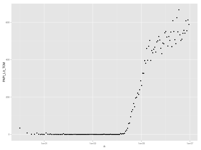
どのレベルのキャッシュも大きな Hash で miss が増えており、とくに L3 は TLB miss と傾向が似ているが、TLB miss が起きるときには cache miss も起こると思うのでそんなものだろう。たぶん。

2016-10-14 (Fri)

#1 cache miss の数

TLB miss が (ほとんど) 起きない程度の領域で、cache miss がどうなっているか数えてみた。

% ./ruby -rPAPI -e '
events = %w[PAPI_L1_DCM PAPI_L2_DCM PAPI_L3_TCM]
evset = PAPI::EventSet.new
evset.add_named(events)
def fmt(n) "%10d" % n end
puts "n,i,t[s],#{events.join(",")}"
n = 1
h = {}
while n < 1e3
  h[fmt(h.size)] = true while h.size < n
  100.times {|i|
    k = fmt(rand(n))
    GC.start
    GC.disable
    h[k]
    t1 = Process.clock_gettime(Process::CLOCK_THREAD_CPUTIME_ID)
    evset.start
    h[k]
    evrec = evset.stop
    t2 = Process.clock_gettime(Process::CLOCK_THREAD_CPUTIME_ID)
    GC.enable
    t = t2-t1
    puts [n,i,t,*evrec].join(",")
    STDOUT.flush
  }
  n = (n*1.1).to_i+1
end' > hash-lookup-cache2.csv

実行時間はほぼ一定に見える。

hash-lookup2-time.png

L1 data cache miss はほぼ一定な感じ。

hash-lookup2-l1dcm.png

L2 data cache miss は最後のほうで少し増加傾向が見える。

hash-lookup2-l2dcm.png

L3 cache miss はほぼ起きていない。

hash-lookup2-l3tcm.png

ふむ、L2 data cache miss が増えているのに L1 data cache miss が増えていないっていうのはどういうことかな。

#2 TLB miss が原因であることの確認方法

L2 data cache miss が増えていても L3 cache miss が一定なのは、working set が L2 cache に入っていることの確認になっている感じがする。

そういう意味では、(もっと大きいところで) 遅くなっている原因が TLB miss であることを確認するためには、その下のメモリ階層のミスが増えていないことを確認すべきなんだろうな。(TLB をメモリ階層というのは少し変な感じがするけれど。)

page fault を数えるのかなぁ。

papi_avail にはそれっぽいのは見当たらないが、papi_native_avail だと以下のあたりがそれっぽい。

minor fault と major fault って何だったかな、と思って検索すると、おそらく、minor fault が TLB miss で、major fault が実際に disk を読むやつかな。(追記: これはまちがい。TLB miss でも page fault (minor fault or major fault) にならないことがある)

しかし、PAPI で perf::MINOR-FAULTS とかを指定しても 0 になってしまってうまく測定できない。

とりあえず、perf コマンドで以下のようにしてみた。

% perf record -e minor-faults,major-faults ./ruby -e '
def fmt(n) "%10d" % n end
puts "n,t[s]"
n = 1
h = {}
while n < 1e8
  h[fmt(h.size)] = true while h.size < n
  k = fmt(rand(n))
  GC.start
  GC.disable
  h[k]
  t1 = Process.clock_gettime(Process::CLOCK_THREAD_CPUTIME_ID)
  h[k]
  t2 = Process.clock_gettime(Process::CLOCK_THREAD_CPUTIME_ID)
  GC.enable
  t = t2-t1
  puts [n,t].join(",")
  STDOUT.flush
  n = (n*1.1).to_i+1
end'
...
% PAGER=cat perf report --stdio
# To display the perf.data header info, please use --header/--header-only options.
#
# Samples: 195K of event 'minor-faults'
# Event count (approx.): 3042982
#
# Overhead  Command      Shared Object                              Symbol
# ........  .......  .................  ..................................
#
    57.53%     ruby  libc-2.19.so       [.] _int_malloc
    26.96%     ruby  ruby               [.] heap_assign_page
    13.26%     ruby  libc-2.19.so       [.] _int_memalign
     2.22%     ruby  libc-2.19.so       [.] memset
     0.02%     ruby  libc-2.19.so       [.] _int_free
     0.01%     ruby  libc-2.19.so       [.] __memcpy_sse2
     0.00%     ruby  ld-2.19.so         [.] memset
     0.00%     ruby  ld-2.19.so         [.] dl_main
     0.00%     ruby  ld-2.19.so         [.] 0x0000000000001190
     0.00%     ruby  [kernel.kallsyms]  [k] __clear_user
     0.00%     ruby  [kernel.kallsyms]  [k] copy_user_enhanced_fast_string


# Samples: 0  of event 'major-faults'
# Event count (approx.): 0
#
# Overhead  Command  Shared Object  Symbol
# ........  .......  .............  ......
#

こちらだと、minor-faults が 195K回起きているが、major-faults は起きていないことが確認できた。

#3 PAPI で minor-faults を測定

おや、単純なケースでは PAPI で minor-faults を測定できるな。

% ./ruby -rPAPI -e '
ev = PAPI::EventSet.new
ev.add_named(%w[perf::MINOR-FAULTS perf::MAJOR-FAULTS])
ev.start
s = "a" * 4096 * 1024
p ev.stop'
[1026, 0]

しかし、やりたかったケースでは依然として minor-faults (と major-faults) が 0 になる。

% ./ruby -rPAPI -e '
events = %w[perf::MINOR-FAULTS perf::MAJOR-FAULTS]
evset = PAPI::EventSet.new
evset.add_named(events)
def fmt(n) "%10d" % n end
puts "n,t[s],#{events.join(",")}"
n = 1
h = {}
while n < 1e8
  h[fmt(h.size)] = true while h.size < n
  k = fmt(rand(n))
  GC.start
  GC.disable
  h[k]
  t1 = Process.clock_gettime(Process::CLOCK_THREAD_CPUTIME_ID)
  evset.start
  h[k]
  evrec = evset.stop
  t2 = Process.clock_gettime(Process::CLOCK_THREAD_CPUTIME_ID)
  GC.enable
  t = t2-t1
  puts [n,t,*evrec].join(",")
  STDOUT.flush
  n = (n*1.1).to_i+1
end'
n,t[s],perf::MINOR-FAULTS,perf::MAJOR-FAULTS
1,1.3289999999999136e-05,0,0
...
98667908,2.5887999981932808e-05,0,0

うしろの二つの数がぜんぶ 0 になってしまう。

これが正しいとするとなんでかな。もしかして、h[k] を測定の直前に一回実行しているのが理由か?

と思ったが違うな。直前に実行するのをやめても minor-faults は 0 のままだ。

% ./ruby -rPAPI -e '
events = %w[perf::MINOR-FAULTS perf::MAJOR-FAULTS]
evset = PAPI::EventSet.new
evset.add_named(events)
def fmt(n) "%10d" % n end
puts "n,t[s],#{events.join(",")}"
n = 1
h = {}
while n < 1e8
  h[fmt(h.size)] = true while h.size < n
  k = fmt(rand(n))
  GC.start
  GC.disable
  #h[k]
  t1 = Process.clock_gettime(Process::CLOCK_THREAD_CPUTIME_ID)
  evset.start
  h[k]
  evrec = evset.stop
  t2 = Process.clock_gettime(Process::CLOCK_THREAD_CPUTIME_ID)
  GC.enable
  t = t2-t1
  puts [n,t,*evrec].join(",")
  STDOUT.flush
  n = (n*1.1).to_i+1
end'
n,t[s],perf::MINOR-FAULTS,perf::MAJOR-FAULTS
1,1.4233000000002383e-05,0,0
...
98667908,3.0279999975846295e-05,0,0

なんでかなぁ。

調べ直すと、x86 の TLB miss は基本的には hardware で処理されるため、TLB miss が起きたからといって、必ずしも割り込みが起きるわけではないようだ。

perf::MINOR-FAULTS や perf::MAJOR-FAULTS は software event で、Linux kernel 内部で発生するので、割り込みで kernel が動かない限り発生しない。

だから、TLB miss が発生しているが、perf::MINOR-FAULTS や perf::MAJOR-FAULTS が発生しないのはおかしくない。

しかし、x86 における minor faults とは何だろう? TLB miss したとき、page table にちゃんと entry が入っていれば hardware で処理されるので、entry が入っていないときで、disk にはアクセスしなくて済む、という状況だが...

Linux kernel を PERF_COUNT_SW_PAGE_FAULTS_MIN とか VM_FAULT_MAJOR で検索して眺める...

必要なページを他のプロセスが読み込んだときとかか? そういう場合に読み込んだ以外のプロセスの page table の更新は必要になるまでやらないというのはありそうである。

しかし、それは以下で minor-faults が発生する理由にはならない。

perf record -e minor-faults ./miniruby -e 's = "a" * 4096 * 1024 * 1024'

perf report で眺めると、__memcpy_sse2_unaligned で発生しているから、空ページ (0 で埋まったページ) へのアクセスが原因かなぁ。

そうすると、Hash の lookup で minor-fault が発生するのはありえなさそうだな。

結局、大きな Hash の lookup が遅くなるときには TLB miss が増えているが、minor-fault, major-fault は起きていないので、遅くなる原因は TLB miss ということになりそう。

いや、perf::PAGE-FAULTS (PERF_COUNT_SW_PAGE_FAULTS) を測定したほうがいいか。arch/x86/mm/fault.c をみると、PERF_COUNT_SW_PAGE_FAULTS_MAJ と PERF_COUNT_SW_PAGE_FAULTS_MIN のどちらかが起きるときには既に PERF_COUNT_SW_PAGE_FAULTS が起きているから、そちらだけでいいはずだ。実際に試してみた。

% ./ruby -rPAPI -e '
events = %w[PAPI_TLB_DM perf::PAGE-FAULTS]
evset = PAPI::EventSet.new
evset.add_named(events)
def fmt(n) "%10d" % n end
puts "n,t[s],#{events.join(",")}"
n = 1
h = {}
while n < 1e8
  h[fmt(h.size)] = true while h.size < n
  k = fmt(rand(n))
  GC.start
  GC.disable
  h[k]
  t1 = Process.clock_gettime(Process::CLOCK_THREAD_CPUTIME_ID)
  evset.start
  h[k]
  evrec = evset.stop
  t2 = Process.clock_gettime(Process::CLOCK_THREAD_CPUTIME_ID)
  GC.enable
  t = t2-t1
  puts [n,t,*evrec].join(",")
  STDOUT.flush
  n = (n*1.1).to_i+1
end'
n,t[s],PAPI_TLB_DM,perf::PAGE-FAULTS
1,1.72339999999771e-05,48,0
...
98667908,3.352400000267153e-05,74,0

というわけで、PAPI_TLB_DM が増えても perf::PAGE-FAULTS は 0 のままなので、遅くなる原因は TLB miss と考えられる。

2016-10-15 (Sat)

#1 x86 のメモリアクセス

メモリのあるアドレスのデータを読み込みたい場合、以下のような処理が CPU の中で行われる、と理解した。手元で試しつつ断片的な情報をつなぎ合わせて理解した結果なので、正しくないかもしれない。(また、手元の CPU で正しいとしても、他の CPU で正しいとは限らない)

仮想記憶が前提で、ふつうのユーザレベルプログラムが対象なので、アクセスしたいアドレスは論理アドレスで与えられる。

  1. 論理アドレスを物理アドレスにアドレス変換する。(x86 の場合、cache は物理アドレスで管理されているので、cache にアクセスする前に物理アドレスを得る必要がある)
    1. まず TLB によるアドレス変換に挑戦 -> 成功 (TLB hit) したら変換終了。CPU の中の hardware だけで済むので速い。
    2. TLB miss になったら PAPI_TLB_DM++ する。(メモリにある) page table を調べてアドレス変換するのに挑戦 -> 成功したら変換終了。メモリにアクセスするので遅いが、software は動かないのでマシ。(x86 の場合ここは hardware 実装になっている)
    3. page table にエントリが入っていなかった場合、page fault 割り込みがが起きて OS が software で処理を行う。PERF_COUNT_SW_PAGE_FAULTS++
      1. アクセスしたいメモリがすでにメモリ内に存在した場合を minor page fault という。PERF_COUNT_SW_PAGE_FAULTS_MIN++ -> page table にエントリを入れて変換に戻る。disk にアクセスするよりはずっと速い。
      2. アクセスしたいメモリがメモリ内に存在せず、disk などにアクセスする必要がある場合を major page fault という。PERF_COUNT_SW_PAGE_FAULTS_MAJ++ -> disk からメモリに読み込んでその page table entry を作る。disk にアクセスするのでとっても遅い。
  2. 物理アドレスで L1 cache に挑戦 -> hit したらアクセス終了。L1 cache は小さくて速い
  3. L1 miss したら PAPI_L1_DCM++ する。L2 cache に挑戦 -> hit したらアクセス終了。L2 cache は L1 cache よりは遅い
  4. L2 miss したら PAPI_L2_DCM++ する。L3 cache に挑戦 -> hit したらアクセス終了。L3 cache は L2 cache より遅い
  5. L3 miss したら PAPI_L3_TCM++ する。しょうがないのでメモリにアクセスする。メモリにアクセスするので遅い

こういう仮想記憶の話は大学とかで学んでいてもおかしくないはずだが、そういう記憶がない。忘れているのか、講義をとらなかったか。

PAPI_L1_DCM++ とかのカウンタのインクリメントは実際には hardware で実装されていたりするわけだが、てきとうに書いておいた。

L3 だけ TCM なのは papi_avail で PAPI_L3_DCM は使えないと表示されるから。手元の CPU では L3 cache が unified cache で data cache と instruction cache が分かれていないからだと思う。

追記: がちゃぴん先生に TLB walk と L1 access は同時に動作できることを指摘されました。cache の key はアドレスの下位ビットで、アドレス変換は上位ビットの変換で、L1 は小さいためそれらは重なっておらず、同時に動作できる、とのこと。なるほど。 <URL:https://twitter.com/kosaki55tea/status/787807862810562560>

#2 CPU の spec

計測に使ったマシンの CPU の情報を書いておく。

/proc/cpuinfo (の最初のひとつ) は以下のとおり。

processor       : 0
vendor_id       : GenuineIntel
cpu family      : 6
model           : 60
model name      : Intel(R) Core(TM) i7-4770 CPU @ 3.40GHz
stepping        : 3
microcode       : 0x7
cpu MHz         : 3892.601
cache size      : 8192 KB
physical id     : 0
siblings        : 8
core id         : 0
cpu cores       : 4
apicid          : 0
initial apicid  : 0
fpu             : yes
fpu_exception   : yes
cpuid level     : 13
wp              : yes
flags           : fpu vme de pse tsc msr pae mce cx8 apic sep mtrr pge mca cmov pat pse36 clflush dts acpi mmx fxsr sse sse2 ss ht tm pbe syscall nx pdpe1gb rdtscp lm constant_tsc arch_perfmon pebs bts rep_good nopl xtopology nonstop_tsc aperfmperf eagerfpu pni pclmulqdq dtes64 monitor ds_cpl vmx smx est tm2 ssse3 fma cx16 xtpr pdcm pcid sse4_1 sse4_2 x2apic movbe popcnt tsc_deadline_timer aes xsave avx f16c rdrand lahf_lm abm ida arat xsaveopt pln pts dtherm tpr_shadow vnmi flexpriority ept vpid fsgsbase tsc_adjust bmi1 hle avx2 smep bmi2 erms invpcid rtm
bogomips        : 6800.11
clflush size    : 64
cache_alignment : 64
address sizes   : 39 bits physical, 48 bits virtual
power management:

ふむ。これだと cache size は 8192KB というだけで、L1/L2/L3 それぞれの cache size はわからないな。

cpuid というコマンドで詳しい情報が出せるようだ。

% cpuid -1
CPU:
   vendor_id = "GenuineIntel"
   version information (1/eax):
      processor type  = primary processor (0)
      family          = Intel Pentium Pro/II/III/Celeron/Core/Core 2/Atom, AMD Athlon/Duron, Cyrix M2, VIA C3 (6)
      model           = 0xc (12)
      stepping id     = 0x3 (3)
      extended family = 0x0 (0)
      extended model  = 0x3 (3)
      (simple synth)  = Intel Core i5-4000 / i7-4000 / Mobile Core i3-4000 / i5-4000 / i7-4000 / Mobile Core i3-4000 / Mobile Core i5-4000 / Mobile Core i7-4000 / Pentium G3000 / Celeron G1800 / Mobile Pentium 3500U / Mobile Celeron 2900U / Xeon E3-1200 v3 (Haswell), 22nm
   miscellaneous (1/ebx):
      process local APIC physical ID = 0x3 (3)
      cpu count                      = 0x10 (16)
      CLFLUSH line size              = 0x8 (8)
      brand index                    = 0x0 (0)
   brand id = 0x00 (0): unknown
   feature information (1/edx):
      x87 FPU on chip                        = true
      virtual-8086 mode enhancement          = true
      debugging extensions                   = true
      page size extensions                   = true
      time stamp counter                     = true
      RDMSR and WRMSR support                = true
      physical address extensions            = true
      machine check exception                = true
      CMPXCHG8B inst.                        = true
      APIC on chip                           = true
      SYSENTER and SYSEXIT                   = true
      memory type range registers            = true
      PTE global bit                         = true
      machine check architecture             = true
      conditional move/compare instruction   = true
      page attribute table                   = true
      page size extension                    = true
      processor serial number                = false
      CLFLUSH instruction                    = true
      debug store                            = true
      thermal monitor and clock ctrl         = true
      MMX Technology                         = true
      FXSAVE/FXRSTOR                         = true
      SSE extensions                         = true
      SSE2 extensions                        = true
      self snoop                             = true
      hyper-threading / multi-core supported = true
      therm. monitor                         = true
      IA64                                   = false
      pending break event                    = true
   feature information (1/ecx):
      PNI/SSE3: Prescott New Instructions     = true
      PCLMULDQ instruction                    = true
      64-bit debug store                      = true
      MONITOR/MWAIT                           = true
      CPL-qualified debug store               = true
      VMX: virtual machine extensions         = true
      SMX: safer mode extensions              = true
      Enhanced Intel SpeedStep Technology     = true
      thermal monitor 2                       = true
      SSSE3 extensions                        = true
      context ID: adaptive or shared L1 data  = false
      FMA instruction                         = true
      CMPXCHG16B instruction                  = true
      xTPR disable                            = true
      perfmon and debug                       = true
      process context identifiers             = true
      direct cache access                     = false
      SSE4.1 extensions                       = true
      SSE4.2 extensions                       = true
      extended xAPIC support                  = true
      MOVBE instruction                       = true
      POPCNT instruction                      = true
      time stamp counter deadline             = true
      AES instruction                         = true
      XSAVE/XSTOR states                      = true
      OS-enabled XSAVE/XSTOR                  = true
      AVX: advanced vector extensions         = true
      F16C half-precision convert instruction = true
      RDRAND instruction                      = true
      hypervisor guest status                 = false
   cache and TLB information (2):
      0x63: data TLB: 1G pages, 4-way, 4 entries
      0x03: data TLB: 4K pages, 4-way, 64 entries
      0x76: instruction TLB: 2M/4M pages, fully, 8 entries
      0xff: cache data is in CPUID 4
      0xb5: instruction TLB: 4K, 8-way, 64 entries
      0xf0: 64 byte prefetching
      0xc1: L2 TLB: 4K/2M pages, 8-way, 1024 entries
   processor serial number: 0003-06C3-0000-0000-0000-0000
   deterministic cache parameters (4):
      --- cache 0 ---
      cache type                           = data cache (1)
      cache level                          = 0x1 (1)
      self-initializing cache level        = true
      fully associative cache              = false
      extra threads sharing this cache     = 0x1 (1)
      extra processor cores on this die    = 0x7 (7)
      system coherency line size           = 0x3f (63)
      physical line partitions             = 0x0 (0)
      ways of associativity                = 0x7 (7)
      WBINVD/INVD behavior on lower caches = false
      inclusive to lower caches            = false
      complex cache indexing               = false
      number of sets - 1 (s)               = 63
      --- cache 1 ---
      cache type                           = instruction cache (2)
      cache level                          = 0x1 (1)
      self-initializing cache level        = true
      fully associative cache              = false
      extra threads sharing this cache     = 0x1 (1)
      extra processor cores on this die    = 0x7 (7)
      system coherency line size           = 0x3f (63)
      physical line partitions             = 0x0 (0)
      ways of associativity                = 0x7 (7)
      WBINVD/INVD behavior on lower caches = false
      inclusive to lower caches            = false
      complex cache indexing               = false
      number of sets - 1 (s)               = 63
      --- cache 2 ---
      cache type                           = unified cache (3)
      cache level                          = 0x2 (2)
      self-initializing cache level        = true
      fully associative cache              = false
      extra threads sharing this cache     = 0x1 (1)
      extra processor cores on this die    = 0x7 (7)
      system coherency line size           = 0x3f (63)
      physical line partitions             = 0x0 (0)
      ways of associativity                = 0x7 (7)
      WBINVD/INVD behavior on lower caches = false
      inclusive to lower caches            = false
      complex cache indexing               = false
      number of sets - 1 (s)               = 511
      --- cache 3 ---
      cache type                           = unified cache (3)
      cache level                          = 0x3 (3)
      self-initializing cache level        = true
      fully associative cache              = false
      extra threads sharing this cache     = 0xf (15)
      extra processor cores on this die    = 0x7 (7)
      system coherency line size           = 0x3f (63)
      physical line partitions             = 0x0 (0)
      ways of associativity                = 0xf (15)
      WBINVD/INVD behavior on lower caches = false
      inclusive to lower caches            = true
      complex cache indexing               = true
      number of sets - 1 (s)               = 8191
   MONITOR/MWAIT (5):
      smallest monitor-line size (bytes)       = 0x40 (64)
      largest monitor-line size (bytes)        = 0x40 (64)
      enum of Monitor-MWAIT exts supported     = true
      supports intrs as break-event for MWAIT  = true
      number of C0 sub C-states using MWAIT    = 0x0 (0)
      number of C1 sub C-states using MWAIT    = 0x2 (2)
      number of C2 sub C-states using MWAIT    = 0x1 (1)
      number of C3 sub C-states using MWAIT    = 0x2 (2)
      number of C4 sub C-states using MWAIT    = 0x4 (4)
      number of C5 sub C-states using MWAIT    = 0x0 (0)
      number of C6 sub C-states using MWAIT    = 0x0 (0)
      number of C7 sub C-states using MWAIT    = 0x0 (0)
   Thermal and Power Management Features (6):
      digital thermometer                     = true
      Intel Turbo Boost Technology            = true
      ARAT always running APIC timer          = true
      PLN power limit notification            = true
      ECMD extended clock modulation duty     = true
      PTM package thermal management          = true
      digital thermometer thresholds          = 0x2 (2)
      ACNT/MCNT supported performance measure = true
      ACNT2 available                         = false
      performance-energy bias capability      = false
   extended feature flags (7):
      FSGSBASE instructions                    = true
      IA32_TSC_ADJUST MSR supported            = true
      BMI instruction                          = true
      HLE hardware lock elision                = true
      AVX2: advanced vector extensions 2       = true
      SMEP supervisor mode exec protection     = true
      BMI2 instructions                        = true
      enhanced REP MOVSB/STOSB                 = true
      INVPCID instruction                      = true
      RTM: restricted transactional memory     = true
      QM: quality of service monitoring        = false
      deprecated FPU CS/DS                     = true
      intel memory protection extensions       = false
      AVX512F: AVX-512 foundation instructions = false
      RDSEED instruction                       = false
      ADX instructions                         = false
      SMAP: supervisor mode access prevention  = false
      Intel processor trace                    = false
      AVX512PF: prefetch instructions          = false
      AVX512ER: exponent & reciprocal instrs   = false
      AVX512CD: conflict detection instrs      = false
      SHA instructions                         = false
      PREFETCHWT1                              = false
   Direct Cache Access Parameters (9):
      PLATFORM_DCA_CAP MSR bits = 0
   Architecture Performance Monitoring Features (0xa/eax):
      version ID                               = 0x3 (3)
      number of counters per logical processor = 0x4 (4)
      bit width of counter                     = 0x30 (48)
      length of EBX bit vector                 = 0x7 (7)
   Architecture Performance Monitoring Features (0xa/ebx):
      core cycle event not available           = false
      instruction retired event not available  = false
      reference cycles event not available     = false
      last-level cache ref event not available = false
      last-level cache miss event not avail    = false
      branch inst retired event not available  = false
      branch mispred retired event not avail   = false
   Architecture Performance Monitoring Features (0xa/edx):
      number of fixed counters    = 0x3 (3)
      bit width of fixed counters = 0x30 (48)
   x2APIC features / processor topology (0xb):
      --- level 0 (thread) ---
      bits to shift APIC ID to get next = 0x1 (1)
      logical processors at this level  = 0x2 (2)
      level number                      = 0x0 (0)
      level type                        = thread (1)
      extended APIC ID                  = 3
      --- level 1 (core) ---
      bits to shift APIC ID to get next = 0x4 (4)
      logical processors at this level  = 0x8 (8)
      level number                      = 0x1 (1)
      level type                        = core (2)
      extended APIC ID                  = 3
   XSAVE features (0xd/0):
      XCR0 lower 32 bits valid bit field mask = 0x00000007
      bytes required by fields in XCR0        = 0x00000340 (832)
      bytes required by XSAVE/XRSTOR area     = 0x00000340 (832)
      XCR0 upper 32 bits valid bit field mask = 0x00000000
   YMM features (0xd/2):
      YMM save state byte size                = 0x00000100 (256)
      YMM save state byte offset              = 0x00000240 (576)
   LWP features (0xd/0x3e):
      LWP save state byte size                = 0x00000000 (0)
      LWP save state byte offset              = 0x00000000 (0)
   extended feature flags (0x80000001/edx):
      SYSCALL and SYSRET instructions        = true
      execution disable                      = true
      1-GB large page support                = true
      RDTSCP                                 = true
      64-bit extensions technology available = true
   Intel feature flags (0x80000001/ecx):
      LAHF/SAHF supported in 64-bit mode     = true
      LZCNT advanced bit manipulation        = true
      3DNow! PREFETCH/PREFETCHW instructions = false
   brand = "Intel(R) Core(TM) i7-4770 CPU @ 3.40GHz"
   L1 TLB/cache information: 2M/4M pages & L1 TLB (0x80000005/eax):
      instruction # entries     = 0x0 (0)
      instruction associativity = 0x0 (0)
      data # entries            = 0x0 (0)
      data associativity        = 0x0 (0)
   L1 TLB/cache information: 4K pages & L1 TLB (0x80000005/ebx):
      instruction # entries     = 0x0 (0)
      instruction associativity = 0x0 (0)
      data # entries            = 0x0 (0)
      data associativity        = 0x0 (0)
   L1 data cache information (0x80000005/ecx):
      line size (bytes) = 0x0 (0)
      lines per tag     = 0x0 (0)
      associativity     = 0x0 (0)
      size (Kb)         = 0x0 (0)
   L1 instruction cache information (0x80000005/edx):
      line size (bytes) = 0x0 (0)
      lines per tag     = 0x0 (0)
      associativity     = 0x0 (0)
      size (Kb)         = 0x0 (0)
   L2 TLB/cache information: 2M/4M pages & L2 TLB (0x80000006/eax):
      instruction # entries     = 0x0 (0)
      instruction associativity = L2 off (0)
      data # entries            = 0x0 (0)
      data associativity        = L2 off (0)
   L2 TLB/cache information: 4K pages & L2 TLB (0x80000006/ebx):
      instruction # entries     = 0x0 (0)
      instruction associativity = L2 off (0)
      data # entries            = 0x0 (0)
      data associativity        = L2 off (0)
   L2 unified cache information (0x80000006/ecx):
      line size (bytes) = 0x40 (64)
      lines per tag     = 0x0 (0)
      associativity     = 8-way (6)
      size (Kb)         = 0x100 (256)
   L3 cache information (0x80000006/edx):
      line size (bytes)     = 0x0 (0)
      lines per tag         = 0x0 (0)
      associativity         = L2 off (0)
      size (in 512Kb units) = 0x0 (0)
   Advanced Power Management Features (0x80000007/edx):
      temperature sensing diode      = false
      frequency ID (FID) control     = false
      voltage ID (VID) control       = false
      thermal trip (TTP)             = false
      thermal monitor (TM)           = false
      software thermal control (STC) = false
      100 MHz multiplier control     = false
      hardware P-State control       = false
      TscInvariant                   = true
   Physical Address and Linear Address Size (0x80000008/eax):
      maximum physical address bits         = 0x27 (39)
      maximum linear (virtual) address bits = 0x30 (48)
      maximum guest physical address bits   = 0x0 (0)
   Logical CPU cores (0x80000008/ecx):
      number of CPU cores - 1 = 0x0 (0)
      ApicIdCoreIdSize        = 0x0 (0)
   (multi-processing synth): multi-core (c=4), hyper-threaded (t=2)
   (multi-processing method): Intel leaf 0xb
   (APIC widths synth): CORE_width=4 SMT_width=1
   (APIC synth): PKG_ID=0 CORE_ID=1 SMT_ID=1
   (synth) = Intel Core i5-4000 / i7-4000 / Mobile Core i3-4000 / i5-4000 / i7-4000 (Haswell), 22nm

cache 0 から cache 3 が、L1 data, L1 instruction, L2, L3 かなぁ。L2 は unified cache か。

それぞれのサイズは直接には書いていないが、おそらく (system coherency line size) * (ways of associativity) * (number of sets) だと想像すると、(値が2のべき乗でないのはなにかの都合だろうから2のべき乗に調整して) サイズは以下のようになるかな。

TLB は以下のような出力があるがどう解釈するか。

0x63: data TLB: 1G pages, 4-way, 4 entries
0x03: data TLB: 4K pages, 4-way, 64 entries
0x76: instruction TLB: 2M/4M pages, fully, 8 entries
0xb5: instruction TLB: 4K, 8-way, 64 entries
0xc1: L2 TLB: 4K/2M pages, 8-way, 1024 entries

L2 TLB という名前からすると、TLB も階層化されているのだろうな。

data TLB は huge page と普通の (4K の) ページの 2種類の機構があり、huge page なら 16G, 4K page の場合は 1M の領域を管理できる。

instruction TLB も 2種類なのかなぁ。2M/4M というのはどっちをとればいいかわからないが、4M をとると、32M の領域を管理できる。もうひとつの機構は 4K page で、2048K = 2M の領域を管理できる。

あと、L2 TLB というのがあって、4K page の場合は 32M, 2M page の場合は 16G 管理できる。

どれも 4K page と huge page に分かれているので以下のように整理できるか。

いや、huge page の場合に、data TLB と L2 TLB が両方 16G というのは変な気がする。

追記: がちゃぴん先生に 2M/4M pages というのは x86_64 では 2M の意味と指摘されました。 <URL:https://twitter.com/kosaki55tea/status/787809362139942912>

#3 prefetch? ちがう?

まてよ。h[k] を測っているわけだがる直前に同じ処理を実行しているから、TLB miss はありえなくないか?

それでも TLB miss が起きる可能性があるのは... prefetch とか?

が、PAPI で prefetch 関連のを測ってみても、hash size が大きいほうでとくに増加している感じはしない。

なら、なんだろうか。

2016-10-16 (Sun)

#1 TLB miss の原因が違う?

h[k] を 2回実行して、後のほうを測っていたのだが、3回実行してそれぞれを測ってみた。

% ./ruby -rPAPI -e '
events = %w[ PAPI_TLB_DM perf::PAGE-FAULTS ]
evset = PAPI::EventSet.new
evset.add_named(events)
def fmt(n) "%10d" % n end
puts "n,i,t[s],#{events.join(",")}"
n = 1
h = {}
while n < 1e7
  h[fmt(h.size)] = true while h.size < n
  k = fmt(rand(n))
  GC.start
  GC.disable
  3.times {|i|
    t1 = Process.clock_gettime(Process::CLOCK_THREAD_CPUTIME_ID)
    evset.start
    h[k]
    evrec = evset.stop
    t2 = Process.clock_gettime(Process::CLOCK_THREAD_CPUTIME_ID)
    t = t2-t1
    puts [n,i,t,*evrec].join(",")
    STDOUT.flush
  }
  GC.enable
  n = (n*1.1).to_i+1
end' > hash-lookup-tlb2.csv

hash-lookup-tlb2-time.png

hash-lookup-tlb2-dm.png

これだと、hash の size が大きい場合、i=0 な最初の回で TLB miss が増加していて、i=1,2 ではほとんど増加は見られない。実行時間も、同様に(TLB miss が起き始めた過渡的なところはなにかが起きているが)i=0 で増加しているが、i=1,2 ではほとんど増加しない。

これは最後の回しか測らなかった時の挙動とは異なるので、測ることによって何かが起きている感じがする。

2016-10-17 (Mon)

#1 Hash は O(1) か。(再)

いくらか理解が進んだので、以下のように測定し直した。

ハッシュを大きくしながら測定するのはいままでどおりだが、それぞれの大きさのときに今回は 3回 (key をランダムに変えて) 測定している。測定対象の h[k] を測定前に (測定とは別に) 実行することはしていない。したがって、h[k] の中で cache miss, TLB miss が起きてもおかしくない。

また、測定前に evset.start; evset.stop というのを実行して、PAPI の動作に必要な部分は cache に入っていて h[k] の測定を邪魔しないことを期待している。

% ./ruby -rPAPI -e '
events = %w[PAPI_TOT_CYC PAPI_TOT_INS PAPI_TLB_DM perf::PAGE-FAULTS]
evset = PAPI::EventSet.new
evset.add_named(events)
def fmt(n) "%10d" % n end
puts "n,i,t[s],#{events.join(",")}"
n = 1
h = {}
total = 0
while n < 1e7
  h[fmt(h.size)] = true while h.size < n
  GC.start
  3.times {|i|
    k = fmt(rand(n))
    GC.disable
    evset.start; evset.stop
    t1 = Process.clock_gettime(Process::CLOCK_THREAD_CPUTIME_ID)
    evset.start
    h[k]
    evrec = evset.stop
    t2 = Process.clock_gettime(Process::CLOCK_THREAD_CPUTIME_ID)
    GC.enable
    t = t2-t1
    puts [n,i,t,*evrec].join(",")
    STDOUT.flush
  }
  n = (n*1.1).to_i+1
end' > hash-lookup-tlb3.csv

まず、PAPI_TOT_INS で測定した、実行した命令数をプロットすると、ほとんどは3700〜3750の範囲に入っており、ほぼ一定である。hash table lookup が O(1) であるということを反映しているといえるだろう。(要素数が 6以下の場合は違う感じがするが、それはコードが別だからだろう)

hash-lookup-tlb3-totins.png

次に、実行時間とトータルのサイクル数をプロットすると、以下のようになる。これらはだいたい同じような形だが、hash のサイズがある程度以上大きいと遅くなっていて、どうみても一定ではない。これだけみると、hash table lookup が O(1) というのはなんだったのか、とも感じる。

また、同じサイズの hash に対して 3回測定しているうち、1回め (i=0) はあからさまに遅い。2回めと 3回め (i=1,2) はあまり変わらないように見える。

hash-lookup-tlb3-time.png

hash-lookup-tlb3-totcyc.png

hash が大きくなって、使用メモリが大きくなったときに遅くなるのは cache や仮想記憶の影響が考えられるが、以下のように、遅くなっているあたりで TLB miss が増加しており、かつ、page fault はまったく起きていないことから、TLB miss が原因であると考えられる。

hash-lookup-tlb3-tlbdm.png

hash-lookup-tlb3-pagefaults.png

cache の影響も調べてみるため、以下のように測定した。(本当は 1回で測定できればいいのだが、PAPI でたくさんのイベントを同時に測定しようとするとエラーになるので別に測定している。どうにかならないのかな。)

% ./ruby -rPAPI -e '
events = %w[PAPI_L1_DCM PAPI_L2_DCM PAPI_L3_TCM]
evset = PAPI::EventSet.new
evset.add_named(events)
def fmt(n) "%10d" % n end
puts "n,i,t[s],#{events.join(",")}"
n = 1
h = {}
total = 0
while n < 1e7
  h[fmt(h.size)] = true while h.size < n
  GC.start
  3.times {|i|
    k = fmt(rand(n))
    GC.disable
    evset.start; evset.stop
    t1 = Process.clock_gettime(Process::CLOCK_THREAD_CPUTIME_ID)
    evset.start
    h[k]
    evrec = evset.stop
    t2 = Process.clock_gettime(Process::CLOCK_THREAD_CPUTIME_ID)
    GC.enable
    t = t2-t1
    puts [n,i,t,*evrec].join(",")
    STDOUT.flush
  }
  n = (n*1.1).to_i+1
end' > hash-lookup-cache3.csv

実行時間は以下のとおりで、前と同じ感じである。

hash-lookup-cache3-time.png

L3 cache miss は TLB miss が増え始めるよりもちょっと小さめのところから起きているように見える。L3 cache が 8M で、L2 TLB が (4K page で) 32M だから、というあたりが原因だろうか。

hash-lookup-cache3-l3tcm.png

L1 data cache と L2 data cache の miss は以下のとおりである。これらの miss は hash のサイズにかかわらず全体的に起きている。ただ、hash のサイズが大きくなるにつれて、miss が増加しているように見える。(L2 のプロットのほうがわかりやすい)

hash-lookup-cache3-l1dcm.png

hash-lookup-cache3-l2dcm.png

2016-10-18 (Tue)

#1 cache/TLB のモデル

ああいうグラフになるのは理屈としては正しいのだろうか。

すごく単純化して、hash table lookup が一定の命令数で実装されていて、ほとんどの命令は一定時間で実行されるが、たったひとつの load 命令は cache hit/miss (あるいは TLB hit/miss など) のどちらかで、実行時間が 2種類に変化する、と仮定しよう。

その load 命令が cache hit したときの実行時間を t1, cache miss したときの実行時間を t2 としよう。また、その load 命令以外の実行時間を t0 とする。

実行時間は、cache hit すれば t0 + t1 になるし、cache miss すれば t0 + t2 になる。

hash table のサイズを s, cache のサイズを c としよう。これらは同じ単位とする。

hash table 以外を無視し、s <= c なら常に cache hit し、c < s なら c / s の確率で cache hit する、と仮定しよう。

すると、実行時間の期待値は s <= c ? t0 + t1 : t0 + (c/s) * t1 + (1-c/s) * t2 となる。

t0 = 5, t1 = 1, t2 = 10, c = 32 として、グラフを描いてみる。

hash-lookup-model.png

まぁ、それっぽい形になった気がする。

2016-10-19 (Wed)

#1 モデルと実測値

せっかくモデルを作ったので、実測値に fit させてみよう。i=0 のときは遅くてなにか起きている気がするので、i=1 のデータを使う。

今回のモデルは線形ではないので、nls を使うことにして、以下のようにパラメータを推定できた。なお、t0, t1, t2 の代わりに t01=t0+t1, t02=t0+t2 を使ってパラメータを減らしている。(というか、t0, t1, t2 をそのまま推定しようとしたら singular gradient matrix at initial parameter estimates というエラーが出てしまった)

> d <- read.csv("2016-10/hash-lookup-tlb3.csv")
> d$i <- as.factor(d$i)
> fit <- nls(t.s. ~ ifelse(n < c, t01, (c/n)*t01 + (1-c/n)*t02), start=c(c=1e5, t01=4e-6, t02=5e-6), data=d[d$i==1,])
> fit
Nonlinear regression model
  model: t.s. ~ ifelse(n < c, t01, (c/n) * t01 + (1 - c/n) * t02)
   data: d[d$i == 1, ]
        c       t01       t02
3.299e+04 4.722e-06 5.297e-06
 residual sum-of-squares: 1.617e-11

Number of iterations to convergence: 6
Achieved convergence tolerance: 6.701e-06

データとモデルを重ねてプロットすると以下のようになる。(stat_function のところで、n <- 10 ** x としなければならないのにしばらく悩んだ。また、geom_smooth で nls を使うやり方は結局うまくやる方法がわからなかった。)

hash-lookup-tlb3-fit.R:

library(ggplot2)
d <- read.csv("2016-10/hash-lookup-tlb3.csv")
d$i <- as.factor(d$i)
i <- 1
fit <- nls(t.s. ~ ifelse(n < c, t01, (c/n)*t01 + (1-c/n)*t02), start=c(c=1e5, t01=4e-6, t02=5e-6), data=d[d$i==i,])
c <- coef(fit)[[1]]
t01 <- coef(fit)[[2]]
t02 <- coef(fit)[[3]]
p <- ggplot(d[d$i==i,], aes(n, t.s., color=i)) +
  geom_point() +
  stat_function(fun=function(x) { n <- 10 ** x; ifelse(n <= c, t01, (c/n)*t01 + (1-c/n)*t02) }) +
  scale_x_log10()
print(p)

hash-lookup-tlb3-fit.png

まぁ、理屈からいえばそうかもしれない、という程度だな。とくに左側でデータが直線にそっているとは言い難い。

2016-10-20 (Thu)

#1 モデルと実測値 (再)

もっとデータをとればマシになるかな、ということで、n を 1e8 までにして、各n毎の繰り返しを 10回にしてやりなおしてみた。

今回は実行時間だけしか使わないので PAPI は使わない。

% ./ruby -e '
def fmt(n) "%10d" % n end
puts "n,i,t[s]"
n = 1
h = {}
total = 0
while n < 1e8
  h[fmt(h.size)] = true while h.size < n
  GC.start
  GC.disable
  10.times {|i|
    k = fmt(rand(n))
    t1 = Process.clock_gettime(Process::CLOCK_THREAD_CPUTIME_ID)
    h[k]
    t2 = Process.clock_gettime(Process::CLOCK_THREAD_CPUTIME_ID)
    t = t2-t1
    puts [n,i,t].join(",")
    STDOUT.flush
  }
  n = (n*1.1).to_i+1
end' > hash-lookup-time2.csv

各n毎の、最初の測定 (i=0) が遅いのは変わらない。GC 直後だし、cache に乗っていないところが多いのであろう。

左のほうは直線になっていて理屈どおり。ただし、何回か測定すると、前と同様にずれることもある。

hash-lookup-time2.R:

library(ggplot2)
d <- read.csv("2016-10/hash-lookup-time2.csv")
d$i <- as.factor(d$i)
p <- ggplot(d, aes(n, t.s., color=i)) +
  geom_point() +
  scale_x_log10()
print(p)

hash-lookup-time2.png

最初の測定を除いて fit を行うと以下のような感じ。

hash-lookup-time2-fit.R:

library(ggplot2)
d <- read.csv("2016-10/hash-lookup-time2.csv")
d$i <- as.factor(d$i)
fit <- nls(t.s. ~ ifelse(n < c, t01, (c/n)*t01 + (1-c/n)*t02), start=c(c=1e5, t01=4e-6, t02=5e-6), data=d[d$i!=0,])
c <- coef(fit)[[1]]
t01 <- coef(fit)[[2]]
t02 <- coef(fit)[[3]]
p <- ggplot(d[d$i!=0,], aes(n, t.s., color=i)) +
  geom_point() +
  stat_function(fun=function(x) { n <- 10 ** x; ifelse(n <= c, t01, (c/n)*t01 + (1-c/n)*t02) }) +
  scale_x_log10()
print(p)

hash-lookup-time2-fit.png

まぁ、それなりに測定点がたくさんあるところを通ってはいる。

でも、(右のほうでは) 測定点がばらけすぎている。cache miss (TLB miss も含む) が 0回 or 1回というのはモデルを単純ににしすぎたかな。

cache miss が起こる可能性のあるアクセスが (1回ではなく) m回あって、miss が 0回以上 m回以下 (二項分布で) 発生する、とすれば良くなるかもしれない。そういうふうに miss の数が分布するとすれば、ばらけることは理解できる。

#2 hash table lookup の実行時間の頻度分布

いくつかの n について、t の頻度分布をグラフにしてみた。

頻度分布を測るのはちょっと難しい。測定数と bin の幅を調整しないといけないのだが、幅を小さくすると測定数を大きくしてもそう簡単にはなめらかにならない感じ。以下では、1000回測り、幅は1e-7[s]にしてある。

% ./ruby -e '
def fmt(n) "%10d" % n end
puts "n,i,t[s]"
n = 10000
h = {}
while n < 1e8
  h[fmt(h.size)] = true while h.size < n
  GC.start
  GC.disable
  1000.times {|i|
    k = fmt(rand(n))
    t1 = Process.clock_gettime(Process::CLOCK_THREAD_CPUTIME_ID)
    h[k]
    t2 = Process.clock_gettime(Process::CLOCK_THREAD_CPUTIME_ID)
    t = t2-t1
    puts [n,i,t].join(",")
    STDOUT.flush
  }
  n = n*10
end' > hash-lookup-time-freq.csv

hash-lookup-time-freq.R:

library(ggplot2)
d <- read.csv("2016-10/hash-lookup-time-freq.csv")
d$i <- as.factor(d$i)
d$n <- as.factor(d$n)
p <- ggplot(d[d$i!=0,], aes(t.s., color=n)) +
  geom_freqpoly(binwidth=1e-7) +
  xlab("t[s]") +
  coord_cartesian(c(0,2e-6))
print(p)

hash-lookup-time-freq.png

まぁ、山の形をしているので、いくつもの乱数が足し合わさった結果な気がする。

2016-10-25 (Tue)

#1 TLB miss の分布

この分布は二項分布な気がする。

何回か load を行って、それぞれで hit/miss して、miss の回数を数えるわけで、もし hit/miss の確率が一定で独立なら、二項分布だろう。

確率が確かに一定で独立かというと、そうでないのはわかっている。load 時に cache/TLB miss が起きれば、cache/TLB の中身が変化して、その変化はその後の load に影響を与えるので、明らかに独立でない。でも、一定で独立と近似できたりしないかなぁ、というわけである。

まぁ、試してみよう。

まず、実行時間じゃなくて回数が必要なので、TLB miss の回数を測る。ここでは、PAPI の DTLB_LOAD_MISSES:MISS_CAUSES_A_WALK をつかう。(PAPI_TLB_DM は DTLB_LOAD_MISSES:MISS_CAUSES_A_WALK と DTLB_STORE_MISSES:MISS_CAUSES_A_WALK の和であり、今回は store は基本的にしないので、PAPI_TLB_DM と DTLB_LOAD_MISSES:MISS_CAUSES_A_WALK は基本的には同じはずである。)

% ./ruby -rPAPI -e '
events = %w[DTLB_LOAD_MISSES:MISS_CAUSES_A_WALK]
evset = PAPI::EventSet.new
evset.add_named(events)
def fmt(n) "%10d" % n end
puts "n,i,t[s],#{events.join(",")}"
n = 10000
h = {}
GC.disable
while n < 1e8
  h[fmt(h.size)] = true while h.size < n
  GC.start
  1000.times {|i|
    k = fmt(rand(n))
    Process.clock_gettime(Process::CLOCK_THREAD_CPUTIME_ID)
    evset.start; evset.stop
    t1 = Process.clock_gettime(Process::CLOCK_THREAD_CPUTIME_ID)
    evset.start
    h[k]
    evrec = evset.stop
    t2 = Process.clock_gettime(Process::CLOCK_THREAD_CPUTIME_ID)
    t = t2-t1
    puts [n,i,t,evrec].join(",")
    STDOUT.flush
  }
  n *= 2
end' > hash-lookup-tlb-freq.csv

グラフにすると、hash のサイズが小さいときには左端に鋭い山があったのが、サイズを増やしていくと山がなまりつつ右にずれていくことがわかる。そして、ある程度以上大きくしてもあまり変わらないようにも思える。(もちろん page fault が起き始めれば変わるだろうが)

hash-lookup-tlb-freq.R:

library(ggplot2)
d <- read.csv("2016-10/hash-lookup-tlb-freq.csv")
d$n <- as.factor(d$n)
d$i <- as.factor(d$i)
d$miss <- d$DTLB_LOAD_MISSES.MISS_CAUSES_A_WALK
d$DTLB_LOAD_MISSES.MISS_CAUSES_A_WALK <- NULL
p <- ggplot(d[d$i!=0,], aes(miss, color=n)) +
  geom_freqpoly(binwidth=1) +
  coord_cartesian(c(0,20))
print(p)

hash-lookup-tlb-freq.png

確率pの事象をn回試行する二項分布では、期待値 E[X]=np, 分散Var(X)=np(1-p) になるそうなので、実験結果の平均と分散から試行数n と確率pを求めてみよう。たぶん p=1-Var(X)/E[X], n = E[X]/p で求められるよな。(平均や分散を求める関数が組み込まれているのは便利。)

> library(plyr)
> d <- read.csv("2016-10/hash-lookup-tlb-freq.csv")
> d$n <- as.factor(d$n)
> d$i <- as.factor(d$i)
> d$miss <- d$DTLB_LOAD_MISSES.MISS_CAUSES_A_WALK
> d$DTLB_LOAD_MISSES.MISS_CAUSES_A_WALK <- NULL
> head(d)
      n i      t.s. miss
1 10000 0 3.776e-06    7
2 10000 1 2.858e-06    8
3 10000 2 2.369e-06    5
4 10000 3 2.262e-06    3
5 10000 4 2.380e-06    6
6 10000 5 2.296e-06    2
> binom_p <- function(x) { 1 - var(x) / mean(x) }
> binom_n <- function(x) { mean(x) / binom_p(x) }
> ddply(d[d$i!=0,], .(n), colwise(binom_p, .(miss)))
          n         miss
1     10000 -39.61511252
2     20000   0.10107692
3     40000  -0.02825651
4     80000   0.03137766
5    160000  -0.06389309
6    320000   0.00239858
7    640000   0.10880288
8   1280000   0.08411615
9   2560000   0.05003379
10  5120000   0.06694540
11 10240000   0.03340431
12 20480000   0.08971798
13 40960000   0.08732990
14 81920000   0.06629310
> ddply(d[d$i!=0,], .(n), colwise(binom_n, .(miss)))
          n          miss
1     10000   -0.05152178
2     20000   26.49148463
3     40000 -124.34349243
4     80000  136.15651050
5    160000  -77.56638875
6    320000 2174.71054171
7    640000   50.11312521
8   1280000   66.71265778
9   2560000  114.09707497
10  5120000   87.81602294
11 10240000  177.40004722
12 20480000   63.97535777
13 40960000   66.89394621
14 81920000   90.86954149

plyr は便利だね、とか周回遅れの感想は置いておくと、各 hash size n に対して、確率と試行数を求めているが、あまり安定していない。

やってみる前は、hash size にかかわらず試行数 (load 回数) が一定になり、また、hash size が大きくなるにつれて確率 (miss の率) が大きくなっていくと期待したのだが、そうとは言い難い。

しばらく考えると、二項分布は確率が 0や1に近いときには山が鋭くなるので、今回のように山がなまっていくだけなのは、二項分布として考えると miss の確率が 1 に収束しないことを示している感じがする。しかし、hash table のサイズが大きければ、hash table の内容にランダムなキーでアクセスするのはほぼ確実に miss するようになるというのは間違いではないと感じられる。

ふむ。hash table の根元の構造体からの load とか、ベンチマークの中での load とか、Ruby の実行自体で起こる load とか、hit すると期待される load を無視しているのがいかんのかな。ほぼ確実に hit する部分が hash table のアクセスによって cache/TLB から追い出されることがあるというストーリーはどうだろうか。これであれば hit が消えないし、アクセスするアドレスによって追い出されたり追い出されなかったりして miss の回数がばらけることを説明できる気がする。

2016-10-26 (Wed)

#1 TLB miss の分布 (再)

もっと細かく測定すればなにかわかるかな、ということでやってみた。

% ./ruby -rPAPI -e '
events = %w[DTLB_LOAD_MISSES:MISS_CAUSES_A_WALK]
evset = PAPI::EventSet.new
evset.add_named(events)
def fmt(n) "%10d" % n end
puts "n,i,t[s],#{events.join(",")}"
n = 10000
h = {}
GC.disable
while n < 1e8
  h[fmt(h.size)] = true while h.size < n
  GC.start
  10000.times {|i|
    k = fmt(rand(n))
    Process.clock_gettime(Process::CLOCK_THREAD_CPUTIME_ID)
    evset.start; evset.stop
    t1 = Process.clock_gettime(Process::CLOCK_THREAD_CPUTIME_ID)
    evset.start
    h[k]
    evrec = evset.stop
    t2 = Process.clock_gettime(Process::CLOCK_THREAD_CPUTIME_ID)
    t = t2-t1
    puts [n,i,t,evrec].join(",")
    STDOUT.flush
  }
  n = (n*1.03).to_i + 1
end' > hash-lookup-tlb-freq2.csv

グラフにすると、明確な規則性が読み取れる。

(ところで、read.csv は .csv.gz, .csv.bz2, .csv.xz を直接読めることを始めて知りました。xz の場合に lzma decoding result 10 という警告が出るのがなんですが。)

まず試行数については、最初の予想の一定というのは外れたのだが、ぐいっと上がっている曲線が一定間隔で繰り返されているように見える。(x軸は対数軸なので、一定間隔というのは、一定の倍数を意味する。)

hash-lookup-tlb-freq2-n.R:

library(ggplot2)
library(plyr)
d <- read.csv("2016-10/hash-lookup-tlb-freq2.csv.xz")
d$i <- as.factor(d$i)
d$miss <- d$DTLB_LOAD_MISSES.MISS_CAUSES_A_WALK
d$DTLB_LOAD_MISSES.MISS_CAUSES_A_WALK <- NULL
binom_p <- function(x) { 1 - var(x) / mean(x) }
binom_n <- function(x) { mean(x) / binom_p(x) }
dn <- ddply(d[d$i!=0,], .(n), colwise(binom_n, .(miss)))
p <- ggplot(dn, aes(n, miss)) +
  geom_point() +
  scale_x_log10() +
  coord_cartesian(NULL, c(-10,200)) +
  ylab("estimated number of experiments")
print(p)

hash-lookup-tlb-freq2-n.png

そして、確率についてはやはり同様の周期で、下降する直線が繰り返されているように見える。ただ、この直線は hash のサイズの増加につれて miss率がある程度まで増加して飽和しているように見える。

hash-lookup-tlb-freq2-p.R:

library(ggplot2)
library(plyr)
d <- read.csv("2016-10/hash-lookup-tlb-freq2.csv.xz")
d$i <- as.factor(d$i)
d$miss <- d$DTLB_LOAD_MISSES.MISS_CAUSES_A_WALK
d$DTLB_LOAD_MISSES.MISS_CAUSES_A_WALK <- NULL
binom_p <- function(x) { 1 - var(x) / mean(x) }
binom_n <- function(x) { mean(x) / binom_p(x) }
dp <- ddply(d[d$i!=0,], .(n), colwise(binom_p, .(miss)))
p <- ggplot(dp, aes(n, miss)) +
  geom_point() +
  scale_x_log10() +
  ylab("estimated probability")
print(p)

hash-lookup-tlb-freq2-p.png

あと、そもそも二項分布という想定がおかしいかもしれないので、平均と分散を直接プロットしてみよう。

hash-lookup-tlb-freq2-m.R:

library(ggplot2)
library(plyr)
d <- read.csv("2016-10/hash-lookup-tlb-freq2.csv.xz")
d$i <- as.factor(d$i)
d$miss <- d$DTLB_LOAD_MISSES.MISS_CAUSES_A_WALK
d$DTLB_LOAD_MISSES.MISS_CAUSES_A_WALK <- NULL
dm <- ddply(d[d$i!=0,], .(n), colwise(mean, .(miss)))
p <- ggplot(dm, aes(n, miss)) +
  geom_point() +
  scale_x_log10() +
  ylab("mean of misses")
print(p)

hash-lookup-tlb-freq2-m.png

hash-lookup-tlb-freq2-v.R:

library(ggplot2)
library(plyr)
d <- read.csv("2016-10/hash-lookup-tlb-freq2.csv.xz")
d$i <- as.factor(d$i)
d$miss <- d$DTLB_LOAD_MISSES.MISS_CAUSES_A_WALK
d$DTLB_LOAD_MISSES.MISS_CAUSES_A_WALK <- NULL
dv <- ddply(d[d$i!=0,], .(n), colwise(var, .(miss)))
p <- ggplot(dv, aes(n, miss)) +
  geom_point() +
  scale_x_log10() +
  ylab("variance of misses")
print(p)

hash-lookup-tlb-freq2-v.png

ふむ、二項分布という仮定は悪くはないのかもしれない。細かい周期的な挙動を無視して全体的な傾向だけをみると、平均と分散は両方とも右上がりな傾向なのが、二項分布のパラメータに直すと、右上がりな傾向は確率だけになり、試行数は一定になる感じなので、性質をうまく分離できている気がする。

それはそれとして、この周期的挙動はなんだろうか、と想像すると、もしかすると、hash table の拡張 (と rehash) あたりだろうか?

Ruby の hash table の拡張は倍々にしていく。実験では要素数を 1e4 から 1e8 まで増やしていくので、log2(1e8/1e4)=13.3 ということで、だいたい 13回くらい拡張が起きているはずである。周期的な挙動は12回弱くらいだから、それなりに近い。

でもそのあたりの hash table の中身の状態は測定するのが面倒くさいな。Ruby の上からは調べられないし。

2016-10-28 (Fri)

#1 もっと細かく

細かく測定することに味をしめたので、もっと細かくしてみた。

細かく測定するとデータが大きくなってしまうのが面倒なので、今回は測定段階で平均と分散を計算してしまい、生データは記録しないことにした。あと、せっかくなので小さいサイズから測定しよう。

% ./ruby -rPAPI -e '
events = %w[DTLB_LOAD_MISSES:MISS_CAUSES_A_WALK]
evset = PAPI::EventSet.new
evset.add_named(events)
def fmt(n) "%10d" % n end
puts "n,mean,var"
n = 1
ntimes = 1000000
h = {}
GC.disable
while n < 1e8
  h[fmt(h.size)] = true while h.size < n
  sum = 0
  sqsum = 0
  GC.start
  ntimes.times {|i|
    k = fmt(rand(n))
    evset.start; evset.stop
    evset.start
    h[k]
    evrec = evset.stop
    nev = evrec.first
    sum += nev
    sqsum += nev**2
  }
  mean = sum.to_f / ntimes
  var = sqsum.to_f / ntimes - mean ** 2
  puts "#{n},#{mean},#{var}"
  n = (n*1.01).to_i + 1
end' > hash-lookup-tlb-freq3.csv

ハッシュの要素数に対する TLB miss の平均は以下のようになる。

hash-lookup-tlb-freq3-m.R:

library(ggplot2)
d <- read.csv("2016-10/hash-lookup-tlb-freq3.csv")
p <- ggplot(d, aes(n, mean)) +
  geom_point() +
  scale_x_log10() +
  ylab("mean(miss)")
print(p)

hash-lookup-tlb-freq3-m.png

ハッシュの要素数に対する TLB miss の分散は以下のようになる。

hash-lookup-tlb-freq3-v.R:

library(ggplot2)
d <- read.csv("2016-10/hash-lookup-tlb-freq3.csv")
p <- ggplot(d, aes(n, var)) +
  geom_point() +
  scale_x_log10() +
  ylim(0,10) + ylab("var(miss)")
print(p)

hash-lookup-tlb-freq3-v.png

とくに平均はきれいに測定できた。右側に注目すると、ハッシュの拡張(rehash)による周期的構造がよく現れている。

Ruby におけるハッシュの拡張は、要素が増えていったときに密度が一定以上になったときに起こる。拡張時にはテーブルのサイズを倍にするので、密度は半分に下がる。また、Ruby のハッシュは連鎖法のハッシュテーブルであり、密度に比例した長さのリストが作られる。

検索時にはそのリストをたどる(平均して半分の長さをたどる)ので、密度に比例して load 命令が増える。load が増えれば (リストなので連続したアドレスでもないし) miss が増える。拡張が起きると密度が半分になるので miss がいっきに減る。これが、要素数が倍になる毎の周期性が現れる原因と推測できる。

ただ、周期的挙動よりも大きな範囲での傾向として、平均は右肩上がりの増加傾向が見える。分散にはこの増加傾向は見えない。テーブルのサイズが大きくなるとテーブルへのアクセスで miss が増えるからかなぁ。miss の平均は load 数だけでなく個々の load の miss 率もそれなりに影響するが、miss の分散は load 数のほうが支配的ということだろうか。

#2 ハッシュの拡張

Ruby の Hash の実装の st.c を眺めると、要素数6個までは埋め込んで、それを越えると bin の数が 16, 32, 64, ... となるように拡張していく。ST_DEFAULT_MAX_DENSITY が 5 と定義してあって、rehash 直前には各 bin には (平均) 長さ5のリストがつながっており、rehash直後には半分の長さ 2.5 に落ちる。

要素数で考えると、16*5=80, 32*5=160, 64*5=320, ... というところで挙動が変化するはずである。グラフの目盛をそのように変えてみよう

hash-lookup-tlb-freq3-m2.R:

library(ggplot2)
d <- read.csv("2016-10/hash-lookup-tlb-freq3.csv")
p <- ggplot(d, aes(n, mean)) +
  geom_point() +
  scale_x_log10(breaks = 5*4**(0:12)) +
  ylab("mean(miss)")
print(p)

hash-lookup-tlb-freq3-m2.png

やはりちょうど目盛のところで変化している。

#3 load命令数

命令数全体がほぼ一定であることは前に測定してわかっているので、loadの命令数もほぼ一定であることは容易に想像できる。

しかし、この「ほぼ一定」な中での微妙な違いが miss の違いを発生させているようなので、細かく測ってみよう。PAPI では、PAPI_LD_INS で測れるようだ。

% ./ruby -rPAPI -e '
events = %w[PAPI_LD_INS]
evset = PAPI::EventSet.new
evset.add_named(events)
def fmt(n) "%10d" % n end
puts "n,mean,var"
n = 1
ntimes = 100000
h = {}
GC.disable
while n < 1e8
  h[fmt(h.size)] = true while h.size < n
  sum = sqsum = 0
  GC.start
  ntimes.times {|i|
    k = fmt(rand(n))
    evset.start; evset.stop
    evset.start
    h[k]
    evrec = evset.stop
    nev = evrec.first
    sum += nev
    sqsum += nev**2
  }
  mean = sum.to_f / ntimes
  var = sqsum.to_f / ntimes - mean ** 2
  puts "#{n},#{mean},#{var}"
  n = (n*1.01).to_i + 1
end' > hash-lookup-load.csv

平均をグラフにすると以下のようになる。

hash-lookup-load-m.R:

library(ggplot2)
d <- read.csv("2016-10/hash-lookup-load.csv")
p <- ggplot(d, aes(n, mean)) +
  geom_point() +
  scale_x_log10(breaks = 5*4**(0:12)) +
  ylab("mean(load)")
print(p)

hash-lookup-load-m.png

平均を見ると、なんか上下に分かれているのが奇妙だが、だいたいが1060から1070に収まっているし、下だけみれば1060から1063くらいに収まっていて、一定の範囲に収まっていることが確認できる。値としては 1%以下の範囲なので、ほぼ一定といって差し支えないだろう。

その一定の範囲の中で、loadの増加の繰り返しが見える。この周期はTLB missが起きるようになるよりもずっと小さなハッシュから発生している。まぁ、それほど大きくなくてもハッシュの拡張は起きているからな。

平均の周期的挙動は、だいたい3命令弱くらい増加しては元に戻るという形に見える。

Ruby の st.c には ST_DEFAULT_MAX_DENSITY が 5 と定義してあって、リストの(平均)長さが5を越えると rehash する。なので rehash する直前にはリストの(平均)長さはだいたい 5 で、rehash した直後での(平均)長さはだいたい 2.5 になるはずである。

検索でリストをたどるときはハッシュ値と次の要素へのポインタの 2つは load しないといけなくて、平均的にはリストの半分の長さをたどるので、rehash前後で load は 2 * (5/2 - 2.5/2) = 2.5命令くらいの差があるはず、ということでだいたい理屈どおりの実験結果といえるかな。

あと、要素数が40より小さいところでは、load数が1060を下回っている。おそらくこれはリストが短いのだろう。6要素を越えると bin が 16個のハッシュテーブルが構成されるので、リストの平均長は 7/16=0.43個くらいから始まり、次の拡張は 80要素(平均長80/16=5) となる。40要素(平均長40/16=2.5) まではそれ以降よりも平均長が短いので、そのぶんload命令が少ないと理解できる。

分散をグラフにすると以下のようになる。分散は大きくなることもあったので、両対数にしてみた。

hash-lookup-load-v.R:

library(ggplot2)
d <- read.csv("2016-10/hash-lookup-load.csv")
p <- ggplot(d, aes(n, var)) +
  geom_point() +
  scale_x_log10(breaks = 5*4**(0:12)) +
  scale_y_log10() +
  ylab("var(load)")
print(p)

hash-lookup-load-v.png

分散は、両対数なのでちょっと形が違うように見えるが、平均と同じような感じで、平均が大きくなれば分散も大きくなっているように見える。右端とかですごく分散が大きくなることがある理由はよくわからない。

2016-10-29 (Sat)

#1 cache miss を測る

TLB miss の挙動については納得できた気がするので、cache miss を測ってみよう。

% ./ruby -rPAPI -e '
events = %w[PAPI_L1_DCM PAPI_L2_DCM PAPI_L3_TCM]
evset = PAPI::EventSet.new
evset.add_named(events)
def fmt(n) "%10d" % n end
puts "n,l1,l2,l3"
nn = 1.0
rep = 10000
GC.disable
h = {}
while nn < 1e4
  n = nn.to_i
  h[fmt(h.size)] = true while h.size < n
  l1sum = l2sum = l3sum = 0
  GC.start
  rep.times {|i|
    k = fmt(rand(n))
    evset.start; evset.stop
    evset.start
    h[k]
    evrec = evset.stop
    l1sum += evrec[0]
    l2sum += evrec[1]
    l3sum += evrec[2]
  }
  l1mean = l1sum.to_f / rep
  l2mean = l2sum.to_f / rep
  l3mean = l3sum.to_f / rep
  puts "#{n},#{l1mean},#{l2mean},#{l3mean}"
  nn = nn*1.001
end'

L1, L2, L3 の miss を数えている。ハッシュの要素数 n を 1 から 1e4 まで増やしながら、それぞれの n について cache miss の数を数えるのを10000回繰り返して平均を出力している。

グラフにすると、どうも不安定なので、3回測ってみた。(上記のプログラムを 3回動かしてみた。)

L1 cache miss の測定結果が以下の3つである。まず、全体に値がばらけている。(平均をとっているにもかかわらず、である。) 80〜160あたりまでは増加傾向で、その後はあまり変わらないもしくは小さな増加傾向という感じかな。ハッシュの拡張 (80, 160, 320, ...) でのずれもあるが、そうでないところでずれることがある。

hash-lookup-cache-1-l1.png

hash-lookup-cache-2-l1.png

hash-lookup-cache-3-l1.png

L2 cache miss の測定結果が以下の3つである。100〜400あたりまでは素直に増加している。その後も大きく見れば増加傾向がさらに増しているが、ふたつの線のあいだをいったりきたりしているように見える。いったりきたりしているところは、3つの測定で異なることが多い。ハッシュの拡張 (80, 160, 320, ...) でのずれもあるが、そうでないところでずれることがある。

hash-lookup-cache-1-l2.png

hash-lookup-cache-2-l2.png

hash-lookup-cache-3-l2.png

L3 cache miss の測定結果が以下の3つである。おおざっぱな形はどれも同じで、右端で急激に増加している。ただ、ここでもふたつの線の間をいったりきたりしているような感じである。いったりきたりしているところは、3つの測定で異なることが多い。

hash-lookup-cache-1-l3.png

hash-lookup-cache-2-l3.png

hash-lookup-cache-3-l3.png

2016-10-30 (Sun)

#1 アドレスをなるべく固定してみる

同じプログラムを動かしても毎回グラフが変わるというのは、毎回変化する要素がどこかにあるということである。

そういう要素はなんとか制御して固定するか、あるいは、制御できないものとして無視して測定したい。

キャッシュの話なので、さまざまなメモリのアドレスが問題ではないかという気がする。具体的には、ふたつの要因が考えられる。ASLR (address space layout randomization) と、Ruby のハッシュ関数である。

どちらも起動毎に異なる動作をする。

Linux で ASLR は以下のようにして設定で抑制できる。(0 に変える前は 2 だった。)

# echo 0 > /proc/sys/kernel/randomize_va_space

追記: がちゃぴん先生が教えてくれたのですが、以下のようにして ASLR をプロセス単位に抑制できるそうです。こっちのほうが限定的に抑制できていいですね。 <URL:https://twitter.com/kosaki55tea/status/792943771948154880>

setarch --addr-no-randomize a.out

(現在使っている) Ruby のハッシュ関数は SipHash だが、これには種を与えることができて、種はプロセスが起動するときにランダムに決定する。これを固定するにはソースを変更する必要がある。まぁ、fill_random_seed から種をゼロクリアした以降のコードを取り除くだけである。

% svn diff --diff-cmd diff -x '-u -p'
Index: random.c
===================================================================
--- random.c	(revision 56525)
+++ random.c	(working copy)
@@ -552,6 +552,7 @@ fill_random_seed(uint32_t *seed, size_t

     memset(seed, 0, len);

+/*
     fill_random_bytes(seed, len, TRUE);

     gettimeofday(&tv, 0);
@@ -565,6 +566,7 @@ fill_random_seed(uint32_t *seed, size_t
 #if SIZEOF_VOIDP > SIZEOF_INT
     seed[2] ^= (uint32_t)((VALUE)&seed >> SIZEOF_INT * CHAR_BIT);
 #endif
+*/
 }

 static VALUE

そうやってなるべく固定的に動作するようにすると、以下のように String#hash, Object#object_id, rand が毎回同じ値になるようになった。

% ./ruby -e 'p "".hash'
1543336582023656316
% ./ruby -e 'p "".hash'
1543336582023656316
% ./ruby -e 'p "".hash'
1543336582023656316
% ./ruby -e 'p Object.new.object_id'
46912500431520
% ./ruby -e 'p Object.new.object_id'
46912500431520
% ./ruby -e 'p Object.new.object_id'
46912500431520
% ./ruby -e 'p rand'
0.42843998755088286
% ./ruby -e 'p rand'
0.42843998755088286
% ./ruby -e 'p rand'
0.42843998755088286

測定プログラムは前回と同じなので省略する。前回同様、3回測定を行った。

L1 cache miss の測定結果が以下の3つである。それなりに似ているが、違うところもけっこうある感じである。

hash-lookup-cache-fixed1-l1.png

hash-lookup-cache-fixed2-l1.png

hash-lookup-cache-fixed3-l1.png

L2 cache miss の測定結果が以下の3つである。かなり似ている。少なくともアドレスを固定しなかったときに比べればはるかに似ている。でも、違う感じなところもある。

hash-lookup-cache-fixed1-l2.png

hash-lookup-cache-fixed2-l2.png

hash-lookup-cache-fixed3-l2.png

L3 cache miss の測定結果が以下の3つである。かなり似ている。ずれも一致しているところが多い。

hash-lookup-cache-fixed1-l3.png

hash-lookup-cache-fixed2-l3.png

hash-lookup-cache-fixed3-l3.png

測定結果が毎回異なる理由は、アドレスの変化がかなり大きな部分を占めている感じがする。

2016-10-31 (Mon)

#1 アドレスを固定しない

アドレスの変化で性能がいろいろ変わるというのはわかったが、普通は (少なくとも Ruby を使う状況では) 狙ったアドレスのメモリを使えるわけではないので、アドレスを選べないことを前提にして平均的な性能に着目するほうが現実的だろう。

(というわけで /proc/sys/kernel/randomize_va_space は 2 に戻して、ruby もソースを変更していないものに戻した。)

そういう性能を測るにはどうすっかな、と考えて、ハッシュをなるべく作り直すことにした。

いままでは最初に空ハッシュを作って、そのハッシュに少しずつ要素を加えながら測定していたのだが、これだと最初のころに加えられた連鎖法のリストの要素のアドレスはずっと変化しない。ハッシュを作り直せばリストも新しく作られて各要素のアドレスも変わるだろう。そうやって変えていけば、異なるサイズのハッシュの測定で相互の影響を避けられるだろう。(ただし、この結果、大きなハッシュの測定はとても長い時間がかかるようになるので、あまり大きなハッシュは測定できなくなる。)

さらに、あるサイズのハッシュを10000回ループで測定していたのも 100回ループを100回と分解して、ハッシュを100回作り直すようにした。ループを分解した結果、測定結果は100倍出力されるので、これはR側で平均をとることにしよう。平均の平均になってしまうが、各平均が一定数 (100個) の平均だから全体の平均がちゃんと求められるはずである。これで、ひとつのサイズのハッシュの測定でも、いろんなアドレスの場合を平均できる。

さらに、ハッシュを作り直すということは、小さいほうから順に測定する必要もない。そこで、測定順もランダムにしてみた。

% ./ruby -rPAPI -e '
events = %w[PAPI_L1_DCM PAPI_L2_DCM PAPI_L3_TCM]
evset = PAPI::EventSet.new
evset.add_named(events)
def fmt(n) "%10d" % n end
puts "n,l1,l2,l3"
rep1 = 100
rep2 = 100
nn = 1.0
ns = []
while nn < 1e4
  n = nn.to_i
  ns << n
  nn = nn*1.001
end
ns = ns * rep1
ns.shuffle!
GC.disable
ns.each {|n|
  h = {}
  h[fmt(h.size)] = true while h.size < n
  l1sum = l2sum = l3sum = 0
  GC.start
  rep2.times {|i|
    k = fmt(rand(n))
    evset.start; evset.stop
    evset.start
    h[k]
    evrec = evset.stop
    l1sum += evrec[0]
    l2sum += evrec[1]
    l3sum += evrec[2]
  }
  l1mean = l1sum.to_f / rep2
  l2mean = l2sum.to_f / rep2
  l3mean = l3sum.to_f / rep2
  puts "#{n},#{l1mean},#{l2mean},#{l3mean}"
}' > hash-lookup-cache-rand.csv

L1 cache miss は以下のようになった。ハッシュの拡張毎 (80, 160, 320, ...) に miss がいっきに減っては次の拡張まで増加していくという形がよく表れている。

hash-lookup-cache-rand-l1.R:

library(ggplot2)
library(plyr)
d <- read.csv("2016-10/hash-lookup-cache-rand.csv.xz")
dl1 <- ddply(d, .(n), colwise(mean, .(l1)))
p <- ggplot(dl1, aes(n, l1)) +
  geom_point() +
  scale_x_log10(breaks = 5*2**(0:24)) +
  ylab("mean(L1 cache miss)")
print(p)

hash-lookup-cache-rand-l1.png

L2 cache miss は以下のようになった。これもハッシュの拡張毎 (80, 160, 320, ...) に miss が減っては次の拡張まで増加していくという形がよく表れている。

hash-lookup-cache-rand-l2.R:

library(ggplot2)
library(plyr)
d <- read.csv("2016-10/hash-lookup-cache-rand.csv.xz")
dl2 <- ddply(d, .(n), colwise(mean, .(l2)))
p <- ggplot(dl2, aes(n, l2)) +
  geom_point() +
  scale_x_log10(breaks = 5*2**(0:24)) +
  ylab("mean(L2 cache miss)")
print(p)

hash-lookup-cache-rand-l2.png

L3 cache miss は以下のようになった。5120でmissが減っているのはハッシュの拡張によるものかもしれないが、それより小さい部分でははっきりしない。あと、1280と2560直後でmissがいったん減ってから増加する傾向なのは奇妙である。

hash-lookup-cache-rand-l3.R:

library(ggplot2)
library(plyr)
d <- read.csv("2016-10/hash-lookup-cache-rand.csv.xz")
dl3 <- ddply(d, .(n), colwise(mean, .(l3)))
p <- ggplot(dl3, aes(n, l3)) +
  geom_point() +
  scale_x_log10(breaks = 5*2**(0:24)) +
  ylab("mean(L3 cache miss)")
print(p)

hash-lookup-cache-rand-l3.png

あと、6要素までとそれ以降で傾向が異なるのも L1, L2, L3 すべてのグラフでみてとれる。6要素までは線形探索なのでまた違うのだろう。その部分で、なんで L1, L3 が増加傾向で、L2 が減少傾向なのかはわからないが。

まぁ、いろいろ工夫して測定すれば、L1, L2 cache についても 連鎖法ハッシュ表というアルゴリズムの性質が表れたグラフを描くことが可能であることがわかった。

#2 もうちょっと大きなところまで測ってみる

L3 cache miss についてはちょうどハッシュの拡張による影響が表れ始めたところで測定が終わっていて、繰り返しというのは苦しいので、もうちょっと大きなところまで測ってみた。

% ./ruby -rPAPI -e '
events = %w[PAPI_L1_DCM PAPI_L2_DCM PAPI_L3_TCM]
evset = PAPI::EventSet.new
evset.add_named(events)
def fmt(n) "%10d" % n end
puts "n,l1,l2,l3"
rep1 = 100
rep2 = 100
nn = 1.0
ns = []
while nn < 2e4
  ns << nn.to_i
  nn = nn*1.001
end
ns = ns * rep1
ns.shuffle!
GC.disable
ns.each {|n|
  h = {}
  h[fmt(h.size)] = true while h.size < n
  l1sum = l2sum = l3sum = 0
  GC.start
  rep2.times {|i|
    k = fmt(rand(n))
    evset.start; evset.stop
    evset.start
    h[k]
    evrec = evset.stop
    l1sum += evrec[0]
    l2sum += evrec[1]
    l3sum += evrec[2]
  }
  l1mean = l1sum.to_f / rep2
  l2mean = l2sum.to_f / rep2
  l3mean = l3sum.to_f / rep2
  puts "#{n},#{l1mean},#{l2mean},#{l3mean}"
}' > hash-lookup-cache-rand2.csv

L1 cache miss は以下のようになった。同じような結果だが、右端で増加が加速している感じなのが面白い。

hash-lookup-cache-rand2-l1.R:

library(ggplot2)
library(plyr)
d <- read.csv("2016-10/hash-lookup-cache-rand2.csv.xz")
dl1 <- ddply(d, .(n), colwise(mean, .(l1)))
p <- ggplot(dl1, aes(n, l1)) +
  geom_point() +
  scale_x_log10(breaks = 5*2**(0:24)) +
  ylab("mean(L1 cache miss)")
print(p)

hash-lookup-cache-rand2-l1.png

L2 cache miss は以下のようになった。前と同じような結果だと思う。

hash-lookup-cache-rand2-l2.R:

library(ggplot2)
library(plyr)
d <- read.csv("2016-10/hash-lookup-cache-rand2.csv.xz")
dl2 <- ddply(d, .(n), colwise(mean, .(l2)))
p <- ggplot(dl2, aes(n, l2)) +
  geom_point() +
  scale_x_log10(breaks = 5*2**(0:24)) +
  ylab("mean(L2 cache miss)")
print(p)

hash-lookup-cache-rand2-l2.png

L3 cache miss は以下のようになった。やはり、5120 の次に 10240 でも miss が減るので、ハッシュの拡張が見えているのだと思う。

hash-lookup-cache-rand2-l3.R:

library(ggplot2)
library(plyr)
d <- read.csv("2016-10/hash-lookup-cache-rand2.csv.xz")
dl3 <- ddply(d, .(n), colwise(mean, .(l3)))
p <- ggplot(dl3, aes(n, l3)) +
  geom_point() +
  scale_x_log10(breaks = 5*2**(0:24)) +
  ylab("mean(L3 cache miss)")
print(p)

hash-lookup-cache-rand2-l3.png

というわけで、L1, L2, L3 cache について、連鎖法ハッシュ表というアルゴリズムの性質が表れた cache miss のグラフを描くことが可能であることがわかった。

#3 cache size

ところで、cache のサイズはどうだったかというと、以下のとおりである。(line-size * number-of-ways * number-of-sets)

で、Ruby の st.h や st.c をみると、ハッシュ表の根元の構造体は st_table というもので、以下のように定義されている。この構造体自体はハッシュ表毎にひとつで、ハッシュ表の要素数 n には依存しない。

struct st_table {
    const struct st_hash_type *type;
    st_index_t num_bins;
    unsigned int entries_packed : 1;
    st_index_t num_entries : ST_INDEX_BITS - 1;
    union {
        struct {
            struct st_table_entry **bins;
            void *private_list_head[2];
        } big;
        struct {
            struct st_packed_entry *entries;
            st_index_t real_entries;
        } packed;
    } as;
};

今考えている連鎖法の部分は big のところ (packed のところではない) である。bins が st_table_entry へのポインタの配列で、この配列は bin 毎に 1 word 消費される。連鎖法のリストの長さは 2.5 から 5 までをいったりきたりするので、中央の (2.5+5)/2=3.75 をとると、bins は n / 3.75 word の長さになる。

連鎖法のリストの要素である st_table_entry は以下のように定義されている。

struct st_table_entry {
    st_index_t hash;
    st_data_t key;
    st_data_t record;
    st_table_entry *next;
    struct list_node olist;
};

list_node は ccan/list/list.h に定義されていて、2 word である。

struct list_node
{
        struct list_node *next, *prev;
};

というわけで、st_table_entry は 6 word である。

昔、がちゃぴん先生のmalloc動画を見た記憶によれば、glibc の malloc はヘッダに 1 word 使っていたような気がする。とすると、st_table_entry を malloc すると 7 word となる。つまり、全体としては 7n word となる。

つまり 1要素あたり (7 + 1/3.75)n = 7.27n word となり、64bit 環境では 1 word が 8 byte なので、58.1 byte である。

cache の line size は 64 byte なので、それよりは少し小さい。

と、考えていいのだろうか。多すぎる気がする。L3 cache miss の測定では 5120でキャッシュの拡張によるmissの減少が観測されており、そのあたりで L3 cache からあふれていると考えられるので、なにか計算をまちがえている気がする。

key に(短い)文字列を使っていて、ひとつの文字列は 5 word (Ruby の 1 object) 消費するというのを考えても 8192*1024/((7+1/3.75+5)*8)=85482で、まだまだ大きい。(それに、ほとんどはhash値の不一致になるから、文字列のkeyにはほとんどアクセスしないと思うし。)


[latest]


田中哲